Abstract
Medical AI models increasingly fuse multiple imaging modalities — CT scans, MRI sequences, and clinical records — to make high-stakes decisions. This workshop teaches you to explain such multi-modal models using Captum, PyTorch’s interpretability library. You will build three complete XAI pipelines covering Classification (Image + Tabular), Regression (Image + Image), and Segmentation (Image + Image → Mask), all on procedurally generated data with known ground-truth signal locations so explanations can be visually verified.
All the code can be find inside this repo : https://


Multi-Modal Explainability (XAI) for Medical Imaging with Captum
Author: Rachid ZEGHLACHE · AI Researcher
Table of Contents
Section 1 — Environment Setup & Imports
# [RUN ONCE] Install dependencies
# Force-reinstall numpy first to avoid ABI binary incompatibility errors,
# then install the remaining packages against the fresh numpy build.
import subprocess, sys

def pip(*args):
    subprocess.check_call([sys.executable, "-m", "pip", *args])

pip("install", "--upgrade", "numpy", "--quiet")
pip("install", "--upgrade", "captum", "torchvision", "seaborn", "scikit-learn", "scipy", "--quiet")

print("All dependencies installed. Please restart the kernel/runtime, then re-run from cell 2 onward.")
All dependencies installed. Please restart the kernel/runtime, then re-run from cell 2 onward.
import torch
import torch.nn as nn
import torch.nn.functional as F
import numpy as np
import matplotlib.pyplot as plt
import seaborn as sns
import warnings
warnings.filterwarnings("ignore")

from captum.attr import (
    IntegratedGradients,
    DeepLift,
    GradientShap,
    Saliency,
    Occlusion,
    FeatureAblation,
    LayerGradCam,
    LayerAttribution,
)

DEVICE = torch.device("cuda" if torch.cuda.is_available() else "cpu")
SEED = 42
torch.manual_seed(SEED)
np.random.seed(SEED)
print(f"Using device: {DEVICE}")
Using device: cpu
Section 2 — XAI Theory & Taxonomy
Overview: This section introduces Explainable AI (XAI) concepts, families of methods, and why they matter in medical imaging.
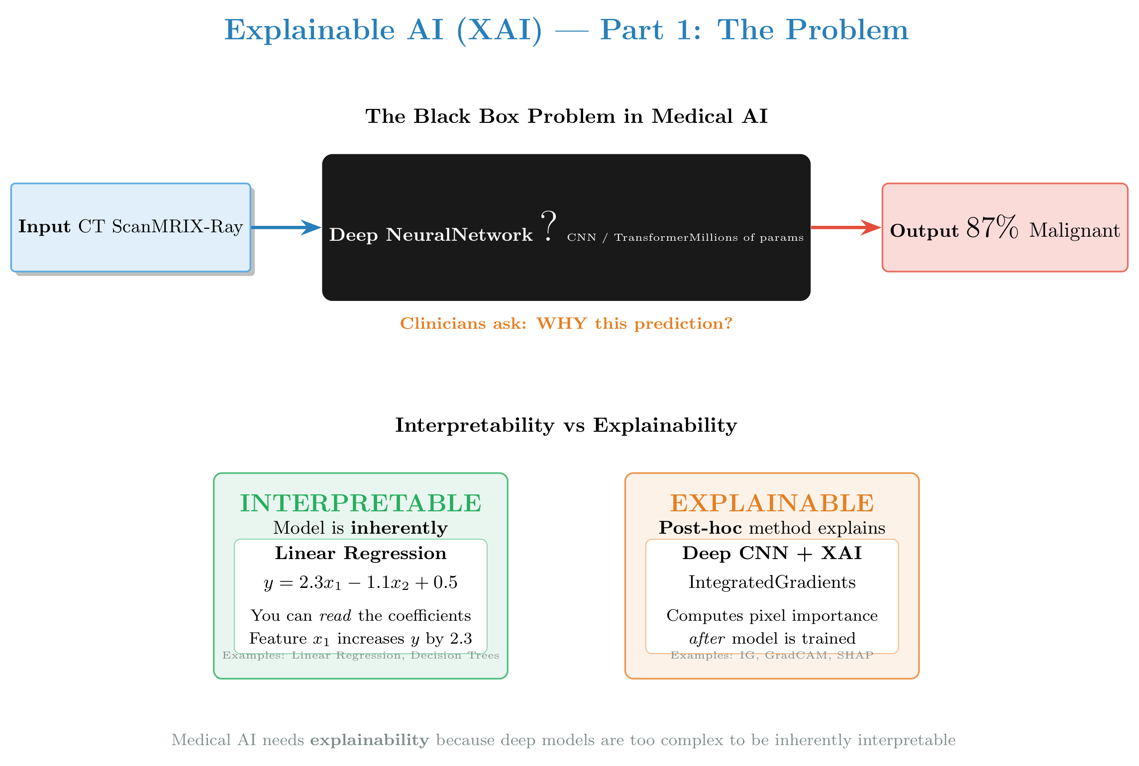
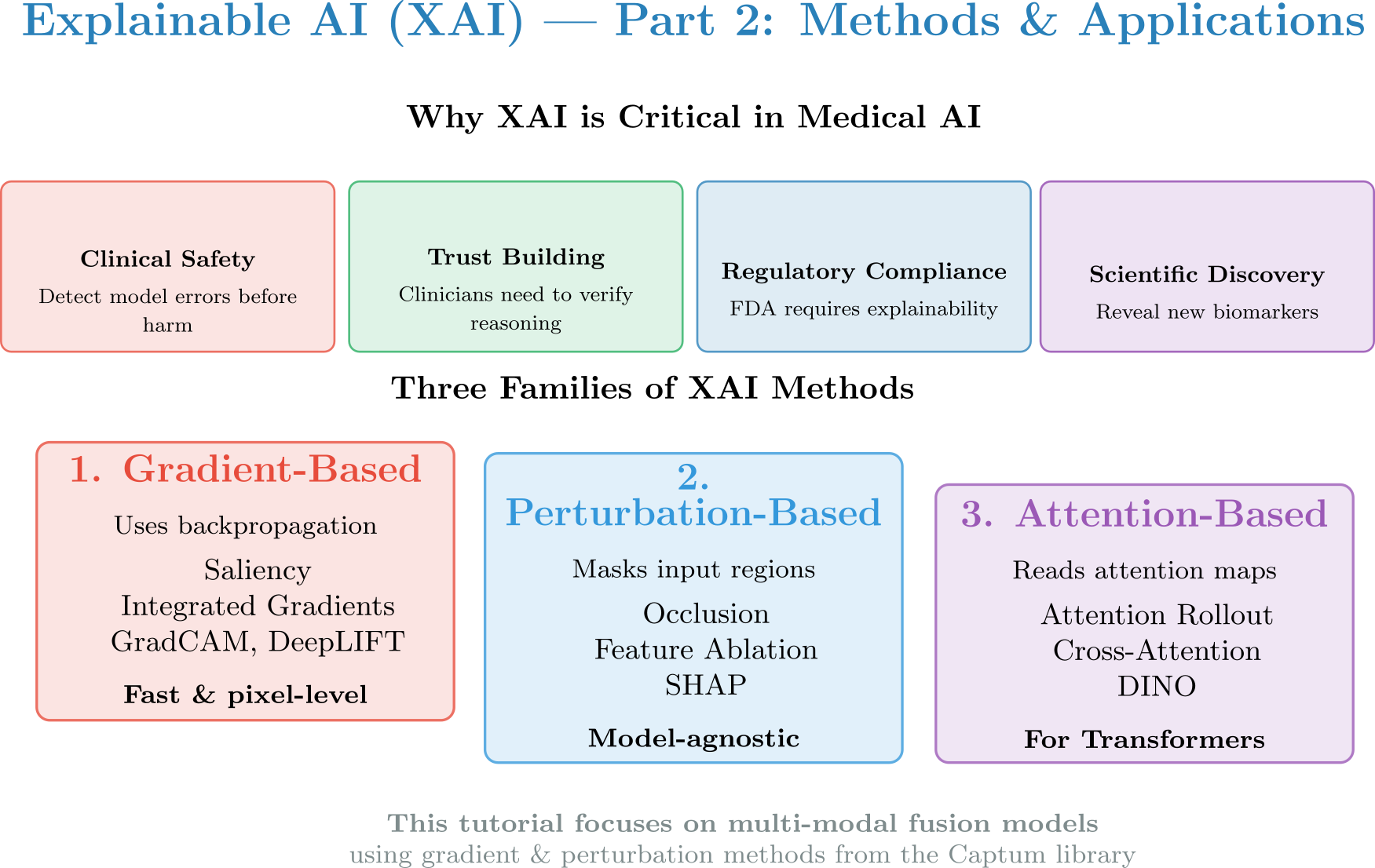
Figure: Comprehensive introduction to XAI — the black box problem, interpretability vs explainability, why XAI is critical in medicine, and the three families of XAI methods we’ll explore in this tutorial.
2.0 — Interpretability vs Explainability
These two terms are often confused but are fundamentally different (see figure above):
| Concept | Definition | Example |
|---|---|---|
| Interpretability | The model is inherently understandable by design | Linear regression, decision tree — you can read the coefficients |
| Explainability | A post-hoc method approximates why a black-box model predicted X | IG on a CNN — explains a single prediction after the fact |
Deep networks used in medical imaging are not interpretable. We use XAI methods to explain their behavior.
2.1 — Why XAI in Medicine?
Clinical Safety: Detect model errors before harm — verify the model is not relying on spurious correlations
Regulatory Compliance: EU AI Act and FDA guidance mandate explainability for high-risk AI systems
Trust Building: Clinicians need to understand and verify the model’s reasoning before making clinical decisions
Scientific Discovery: XAI can reveal new biomarkers or disease patterns not previously known
2.2 — Family 1: Gradient-Based Methods
Core intuition: “Which pixels, if perturbed slightly, would change the model output the most?”
Mathematically, given a model and input , the saliency is:
This is simply the gradient of the output with respect to the input. A large gradient at pixel means that pixel has a strong influence on the prediction.
Unimodal case
| Method | Idea | Formula |
|---|---|---|
| Saliency | Raw gradient magnitude | |
| Integrated Gradients (IG) | Integrate gradient from baseline to input — satisfies completeness and sensitivity axioms | |
| DeepLIFT | Propagate difference from a reference activation back to inputs | , where |
| GradCAM | Gradient w.r.t. last conv feature map; coarse but class-discriminative | , |
| GradientSHAP | Approximates SHAP values using gradient of noisy samples × (input − baseline) | Stochastic IG variant |
Why IG over raw gradients? Raw gradients suffer from gradient saturation — near a flat region, gradients vanish even if the feature is important. IG fixes this by integrating the path from baseline to input.
Extending to multi-modal (Captum tuple-input API)
When the model takes two inputs , gradients flow through each stream independently:
Captum handles this automatically via the tuple-input API — you get one attribution tensor per modality:
attr_x1, attr_x2 = ig.attribute(
    inputs=(x1, x2),
    baselines=(baseline1, baseline2),
    target=class_idx,
)
You can then compute modality importance as the mean absolute attribution per modality:
2.3 — Family 2: Perturbation-Based Methods
Core intuition: “What happens to the model output when I hide or change parts of the input?”
Instead of computing gradients, these methods probe the model by systematically removing or replacing regions and measuring the output change.
Unimodal case
| Method | Idea |
|---|---|
| Occlusion | Slide a grey/black patch over the image; large output drop = important region |
| Feature Ablation | Zero out entire features (e.g., a tabular column, or a whole modality) |
| LIME | Fit a local linear model on perturbed samples around the input |
| SHAP | Use game-theory Shapley values; computes average marginal contribution of each feature |
Trade-off vs gradient-based: Perturbation methods are model-agnostic (no backprop needed) but are much slower — every probe requires a forward pass. Occlusion on a 224×224 image with a 8×8 patch and stride 4 requires ~(55×55) = 3025 forward passes per sample.
Extending to multi-modal
Perturbation-based methods extend naturally: you can ablate at the modality level by zeroing an entire input tensor.
# Feature Ablation — assign each modality its own group ID
mask_t1 = torch.ones_like(t1_xai)          # group 1
mask_t2 = torch.ones_like(t2_xai) * 2      # group 2
attr_t1, attr_t2 = fa.attribute(
    inputs=(t1_xai, t2_xai),
    feature_mask=(mask_t1, mask_t2),
)
This gives a single importance score per modality — directly answering “which MRI sequence matters more?”
2.4 — Family 3: Attention-Based Methods
Core intuition: “Where did the model’s Transformer attention heads look?”
Attention-based methods are only applicable when the model contains attention mechanisms (Transformers, Vision Transformers, nnFormer, etc.).
Unimodal case
| Method | Idea |
|---|---|
| Attention maps | Directly visualize multi-head attention weights for the [CLS] token |
| Attention Rollout | Propagate attention matrices through layers (account for residual connections) |
| DINO | Self-supervised attention captures semantic object boundaries without labels |
Extending to multi-modal
For multi-modal Transformers (e.g., MedFuse, BioViL-T), cross-attention layers connect tokens from different modalities. The cross-attention matrix tells you: “how much did modality-B token influence modality-A token ?”
Note: The models in this workshop use CNNs, not Transformers — so attention-based methods do not directly apply here. We cover this family for completeness. GradCAM is often used as an attention-like proxy for CNN models.
2.5 — Multi-Modal Challenge & Captum API
Single-input XAI tells you where a model looked in one image. Multi-modal XAI must also answer:
“How much did each modality (CT vs. EHR, T1 vs. T2, FLAIR vs. T1ce) contribute?”
Captum’s tuple-input API elegantly solves this by treating each modality as a separate input with independent gradient flow:
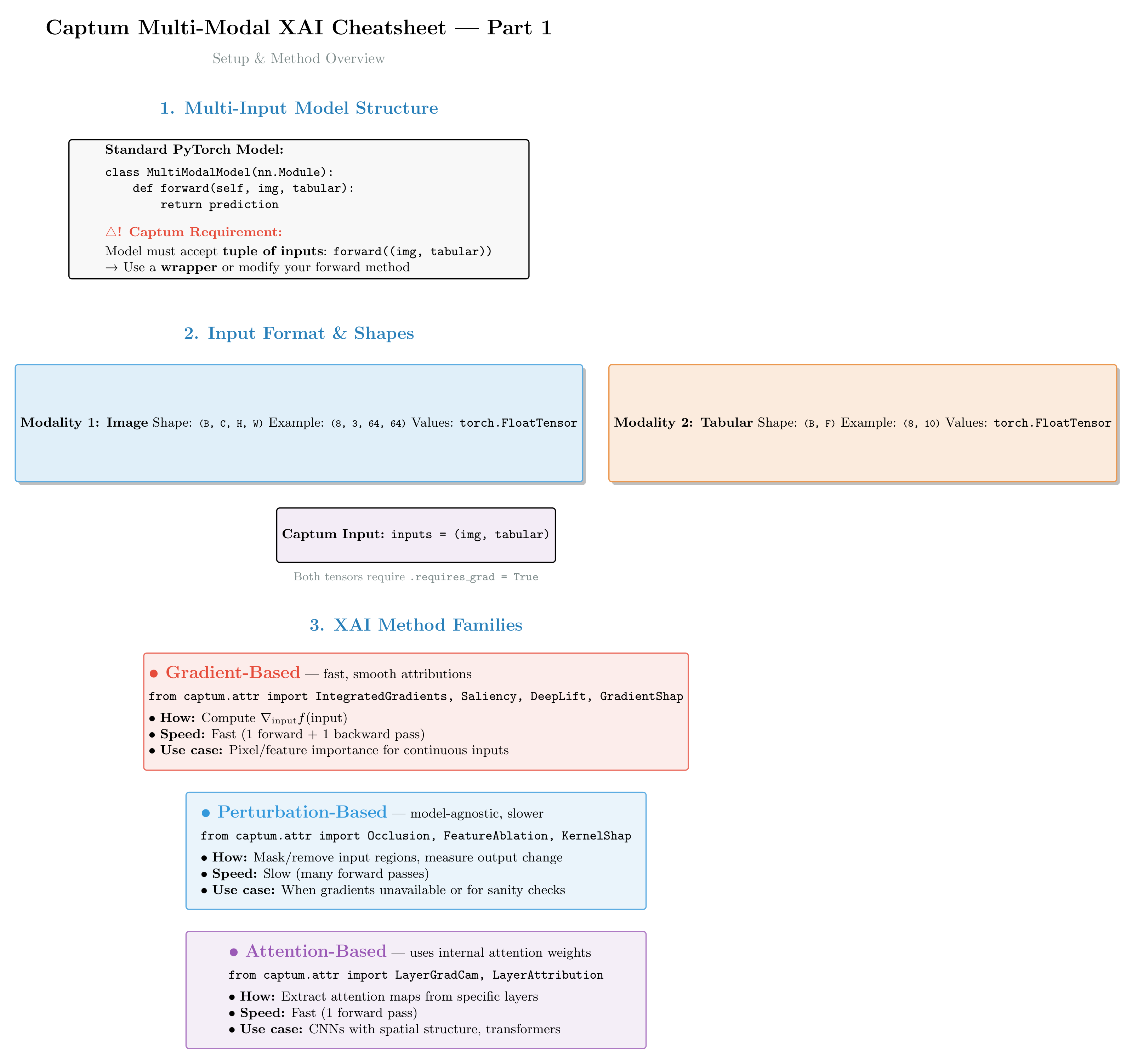
Figure 5a: Captum’s multi-modal API pattern. Each modality gets its own attribution tensor. The inputs tuple structure is mirrored in the outputs — clean and consistent!
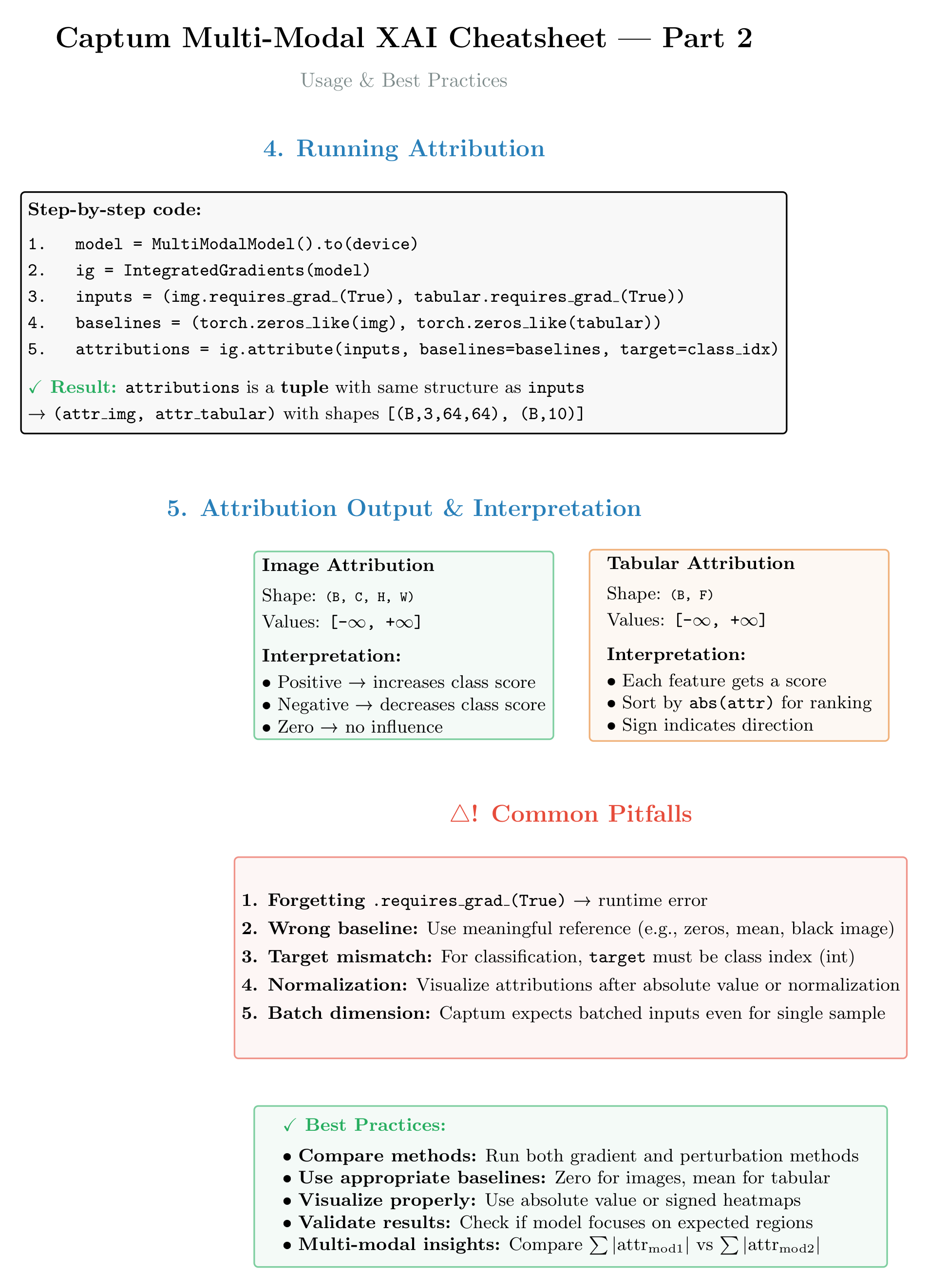
Figure 5b: Quick reference for common Captum methods in multi-modal scenarios. Shows method signatures, when to use each approach, and key parameters (baselines, targets, n_steps).
Core API pattern:
attr1, attr2 = method.attribute(
    inputs=(x1, x2),
    baselines=(b1, b2),
    target=class_idx,   # or None for regression, or 0 for single output
)
Key principles:
Both inputs must have
requires_grad=TrueBaselines should be meaningful references (zeros, dataset mean, blur-masked image)
The
targetparameter specifies which output neuron to explain:Classification: class index (0, 1, 2, ...)
Regression: output neuron index (usually 0 for single-output models)
Segmentation: use a wrapper to reduce spatial output to scalar (e.g., mean probability)
Section 3 — Utility Functions & Model Wrappers
All plotting helpers and Captum-compatibility wrappers live in the standalone module xai_utils.py (in this folder).
This keeps the notebook cells focused on the XAI logic while making the utilities reusable in scripts and tests.
# ── Import shared utilities from xai_utils.py ─────────────────────────────────
import sys, pathlib
sys.path.insert(0, str(pathlib.Path(".").resolve()))

from xai_utils import (
    normalize_attr,
    plot_img_attr,
    plot_tabular_attr,
    plot_modality_importance,
    overlay_attribution,
    plot_dual_attr,
    MultiInputWrapper,
    SegReductionWrapper,
    EHR_FEATURE_NAMES,
    IMG_SIZE,
)
print("xai_utils loaded — utility functions and model wrappers ready.")
xai_utils loaded — utility functions and model wrappers ready.
Section 4 — Realistic Synthetic Data Generation & Loading
All data is procedurally generated by the standalone script generate_dataset.py to faithfully mimic the physical and clinical properties of real medical imaging data, while embedding known ground-truth signals for XAI verification.
This mirrors a real-world workflow where data preparation and model training live in separate stages.
| Task | Modalities | Realism Highlights | Planted Signal |
|---|---|---|---|
| Classification | CT (224×224) + 12 EHR features | Hounsfield-inspired tissue layers, anatomical noise, realistic circular/spiculated nodule | Nodule in left lobe (label=0/benign) or right lobe (label=1/malignant + spiculation); SUVmax, age, pack-years discriminative |
| Regression | T1 MRI + T2 MRI (224×224) | Tissue-contrast T1/T2 relaxation ratios (WM bright T1, CSF dark T1/bright T2), bandpass spatial texture, smooth tissue gradients | WM/CSF T1 signal variation tracks EDSS-like score; periventricular T2 hyperintensity scales with score |
| Segmentation | FLAIR + T1ce (224×224) | Brain parenchyma with sulci/gyri folding texture, realistic ring-enhancing lesion with necrotic core + peritumoral edema | FLAIR: edema halo bright; T1ce: ring-enhancing rim bright, necrotic core dark; mask = full tumor |
import subprocess, pathlib

DATA_DIR = pathlib.Path("data")

if not DATA_DIR.exists() or len(list(DATA_DIR.glob("*.npz"))) < 9:
    print("Running generate_dataset.py  (may take ~2 min on first run) ...")
    subprocess.check_call(
        [sys.executable, "generate_dataset.py",
         "--n", "300", "--seed", "42",
         "--xai_n", "30", "--xai_seed", "999",
         "--out_dir", str(DATA_DIR)],
    )
else:
    print(f"Data directory already populated ({len(list(DATA_DIR.glob('*')))} files). Skipping generation.")

# Verify files exist
expected = [
    "cls_images.npz", "cls_tabular.npz", "cls_metadata.csv",
    "cls_xai_images.npz", "cls_xai_tabular.npz",
    "reg_t1.npz", "reg_t2.npz", "reg_scores.npz",
    "reg_xai_t1.npz", "reg_xai_t2.npz", "reg_xai_scores.npz",
    "seg_flair.npz", "seg_t1ce.npz", "seg_masks.npz",
    "seg_xai_flair.npz", "seg_xai_t1ce.npz", "seg_xai_masks.npz",
]
for f in expected:
    assert (DATA_DIR / f).exists(), f"Missing: {f}"
print(f"All {len(expected)} data files verified in {DATA_DIR}/")
Data directory already populated (17 files). Skipping generation.
All 17 data files verified in data/
4.2 — Constants & helper functions (used throughout the notebook)
from scipy.ndimage import gaussian_filter, label as ndlabel

# -- Tissue & texture helpers (used by EDA visualisation cells) ----------------

def _smooth_noise(rng, shape, scale=0.04, sigma=2.0):
    """Low-frequency perlin-like noise via blurred random field."""
    raw = rng.normal(0, scale, shape).astype(np.float32)
    return gaussian_filter(raw, sigma=sigma)


def _circular_mask(img_size, cx, cy, r):
    y, x = np.ogrid[:img_size, :img_size]
    return ((x - cx)**2 + (y - cy)**2) <= r**2


def _ellipse_mask(img_size, cx, cy, rx, ry, angle_deg=0):
    """Rotated ellipse mask."""
    y, x = np.ogrid[:img_size, :img_size]
    cos_a = np.cos(np.radians(angle_deg))
    sin_a = np.sin(np.radians(angle_deg))
    xr = cos_a * (x - cx) + sin_a * (y - cy)
    yr = -sin_a * (x - cx) + cos_a * (y - cy)
    return (xr**2 / rx**2 + yr**2 / ry**2) <= 1.0


EHR_FEATURE_NAMES = [
    "Age", "PackYears", "SUVmax",
    "NoduleDiam_mm", "SpiculationIdx", "PleuraTether",
    "FEV1_pct", "BMI", "CRP_mgL",
    "FamilyHx", "SmokingStatus", "Gender"
]

IMG_SIZE = 224

print("Helper functions & constants defined.")
Helper functions & constants defined.
Section 5 — Dataset & DataLoader Builders
Each Dataset loads pre-generated data from disk (.npz + .csv files produced by generate_dataset.py) and exposes the standard PyTorch interface.metadata DataFrames are attached to ClsDataset and RegDataset for EDA convenience.
from torch.utils.data import Dataset, DataLoader
import pandas as pd

N_SAMPLES = 300
IMG_SIZE  = 224


class ClsDataset(Dataset):
    """CT + 12-feature EHR binary classification dataset (loaded from disk).

    self.metadata — pd.DataFrame with all EHR features + label for EDA.
    """
    def __init__(self, npz_prefix="cls", data_dir=DATA_DIR):
        img_data = np.load(data_dir / f"{npz_prefix}_images.npz")
        tab_data = np.load(data_dir / f"{npz_prefix}_tabular.npz")
        self.images  = torch.tensor(img_data["images"])           # (N, 1, H, W)
        self.tabular = torch.tensor(tab_data["tabular"])           # (N, 12)
        self.labels  = torch.tensor(tab_data["labels"])            # (N,)
        meta_path = data_dir / f"{npz_prefix}_metadata.csv"
        if meta_path.exists():
            self.metadata = pd.read_csv(meta_path)
        else:
            rows = []
            for i in range(len(self.labels)):
                row = dict(zip(EHR_FEATURE_NAMES, self.tabular[i].numpy()))
                row["Label"] = int(self.labels[i])
                row["LabelName"] = "Malignant" if row["Label"] == 1 else "Benign"
                rows.append(row)
            self.metadata = pd.DataFrame(rows)

    def __len__(self):
        return len(self.labels)

    def __getitem__(self, idx):
        return self.images[idx], self.tabular[idx], self.labels[idx]


class RegDataset(Dataset):
    """T1 + T2 MRI regression dataset (loaded from disk).

    self.scores — list of float scores for EDA.
    """
    def __init__(self, npz_prefix="reg", data_dir=DATA_DIR):
        t1_data   = np.load(data_dir / f"{npz_prefix}_t1.npz")
        t2_data   = np.load(data_dir / f"{npz_prefix}_t2.npz")
        sc_data   = np.load(data_dir / f"{npz_prefix}_scores.npz")
        self.t1     = torch.tensor(t1_data["t1"])             # (N, 1, H, W)
        self.t2     = torch.tensor(t2_data["t2"])             # (N, 1, H, W)
        self.score_tensor = torch.tensor(sc_data["scores"]).float().unsqueeze(1)  # (N, 1)
        self.scores = sc_data["scores"].tolist()

    def __len__(self):
        return len(self.scores)

    def __getitem__(self, idx):
        return self.t1[idx], self.t2[idx], self.score_tensor[idx]


class SegDataset(Dataset):
    """FLAIR + T1ce + lesion mask segmentation dataset (loaded from disk)."""
    def __init__(self, npz_prefix="seg", data_dir=DATA_DIR):
        fl_data = np.load(data_dir / f"{npz_prefix}_flair.npz")
        tc_data = np.load(data_dir / f"{npz_prefix}_t1ce.npz")
        mk_data = np.load(data_dir / f"{npz_prefix}_masks.npz")
        self.flair = torch.tensor(fl_data["flair"])           # (N, 1, H, W)
        self.t1ce  = torch.tensor(tc_data["t1ce"])            # (N, 1, H, W)
        self.masks = torch.tensor(mk_data["masks"])           # (N, 1, H, W)

    def __len__(self):
        return self.flair.shape[0]

    def __getitem__(self, idx):
        return self.flair[idx], self.t1ce[idx], self.masks[idx]


# ── Build datasets from saved files ───────────────────────────────────────────
print("Loading datasets from disk …")
cls_ds  = ClsDataset("cls")
reg_ds  = RegDataset("reg")
seg_ds  = SegDataset("seg")

cls_loader  = DataLoader(cls_ds, batch_size=16, shuffle=True,  num_workers=0)
reg_loader  = DataLoader(reg_ds, batch_size=16, shuffle=True,  num_workers=0)
seg_loader  = DataLoader(seg_ds, batch_size=8,  shuffle=True,  num_workers=0)

# XAI dataloaders (loaded from the separate xai subset files)
cls_xai_ds = ClsDataset("cls_xai")
reg_xai_ds = RegDataset("reg_xai")
seg_xai_ds = SegDataset("seg_xai")
cls_xai_loader = DataLoader(cls_xai_ds, batch_size=1, shuffle=False)
reg_xai_loader = DataLoader(reg_xai_ds, batch_size=1, shuffle=False)
seg_xai_loader = DataLoader(seg_xai_ds, batch_size=1, shuffle=False)

print(f"Datasets ready  —  cls: {len(cls_ds)} | reg: {len(reg_ds)} | seg: {len(seg_ds)} samples")
print(f"XAI subsets     —  cls: {len(cls_xai_ds)} | reg: {len(reg_xai_ds)} | seg: {len(seg_xai_ds)} samples")
print(f"Image resolution: {IMG_SIZE}x{IMG_SIZE}  |  EHR features: {len(EHR_FEATURE_NAMES)}")
Loading datasets from disk …
Datasets ready — cls: 1000 | reg: 1000 | seg: 1000 samples
XAI subsets — cls: 100 | reg: 100 | seg: 100 samples
Image resolution: 224x224 | EHR features: 12
Section 6 — Exploratory Data Analysis (EDA)
Before modelling we inspect the three datasets across four lenses:
Image montage — visual quality & modality contrast
Intensity distributions — histogram per tissue/class
Tabular EDA — class-stratified statistics, correlation heatmap
Dataset-level statistics — label balance, lesion size distribution, score distribution
6.1 — Classification: CT + EHR
import matplotlib.patches as mpatches

# ── 6.1a  Image montage ─────────────────────────────────────────────────────
fig, axes = plt.subplots(2, 6, figsize=(18, 6))
# Gather 6 benign and 6 malignant samples from the dataset
benign_idxs  = [i for i in range(len(cls_ds)) if int(cls_ds.labels[i]) == 0][:6]
malig_idxs   = [i for i in range(len(cls_ds)) if int(cls_ds.labels[i]) == 1][:6]
for row, (idxs, lname) in enumerate([(benign_idxs, "Benign"), (malig_idxs, "Malignant")]):
    for k, idx in enumerate(idxs):
        img_t, _, _ = cls_ds[idx]
        axes[row, k].imshow(img_t.squeeze().numpy(), cmap="gray", vmin=0, vmax=1)
        axes[row, k].axis("off")
        if k == 0:
            axes[row, k].set_title(f"CT — {lname}", loc="left", fontweight="bold",
                                    fontsize=10, pad=4)

plt.suptitle("Task A · CT Image Montage  (top: Benign, bottom: Malignant)", fontsize=13, y=1.01)
plt.tight_layout()
plt.show()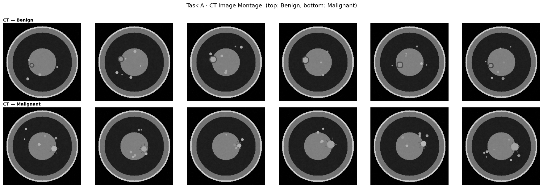
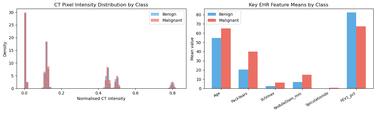
# ── 6.1b  Intensity histograms per class ────────────────────────────────────
fig, axes = plt.subplots(1, 2, figsize=(13, 4))

all_pixels = {0: [], 1: []}
for idx in range(min(60, len(cls_ds))):
    img, _, lbl = cls_ds[idx]
    all_pixels[int(lbl.item())].append(img.numpy().ravel())

colors = {0: "#3498db", 1: "#e74c3c"}
labels = {0: "Benign", 1: "Malignant"}

for lbl, pix_list in all_pixels.items():
    arr = np.concatenate(pix_list)
    axes[0].hist(arr, bins=80, alpha=0.55, color=colors[lbl],
                 label=labels[lbl], density=True)

axes[0].set_xlabel("Normalised CT intensity")
axes[0].set_ylabel("Density")
axes[0].set_title("CT Pixel Intensity Distribution by Class")
axes[0].legend()

# ── 6.1c  EHR class statistics table ──────────────────────────────────────
meta = cls_ds.metadata
stats = meta.groupby("LabelName")[EHR_FEATURE_NAMES[:9]].agg(["mean", "std"])
stats.columns = [f"{f}_{s}" for f, s in stats.columns]
stats_T = stats.T
print(stats_T.to_string())

# Radar / bar comparison for top discriminative features
top_feats = ["Age", "PackYears", "SUVmax", "NoduleDiam_mm", "SpiculationIdx", "FEV1_pct"]
benign_means    = meta[meta.Label == 0][top_feats].mean()
malignant_means = meta[meta.Label == 1][top_feats].mean()

x = np.arange(len(top_feats))
w = 0.35
axes[1].bar(x - w/2, benign_means.values,    w, label="Benign",    color="#3498db", alpha=0.80)
axes[1].bar(x + w/2, malignant_means.values, w, label="Malignant", color="#e74c3c", alpha=0.80)
axes[1].set_xticks(x)
axes[1].set_xticklabels(top_feats, rotation=30, ha="right", fontsize=9)
axes[1].set_ylabel("Mean value")
axes[1].set_title("Key EHR Feature Means by Class")
axes[1].legend()

plt.tight_layout()
plt.show()
LabelName Benign Malignant
Age_mean 54.868460 64.990940
Age_std 7.974023 8.074204
PackYears_mean 20.361829 39.832493
PackYears_std 9.970879 12.313439
SUVmax_mean 2.496799 6.418143
SUVmax_std 0.818092 1.471868
NoduleDiam_mm_mean 7.091237 14.750829
NoduleDiam_mm_std 2.337710 4.899538
SpiculationIdx_mean 0.176652 0.722602
SpiculationIdx_std 0.128126 0.157995
PleuraTether_mean 0.090000 0.402000
PleuraTether_std 0.286468 0.490793
FEV1_pct_mean 82.224398 67.134077
FEV1_pct_std 12.241022 13.691634
BMI_mean 26.393236 24.011906
BMI_std 4.075355 3.994324
CRP_mgL_mean 2.923163 7.568775
CRP_mgL_std 2.915512 7.707013
# ── 6.1d  EHR correlation heatmap ───────────────────────────────────────────
fig, axes = plt.subplots(1, 2, figsize=(16, 5))

for ax, lbl, lname, cmap in zip(axes, [0, 1], ["Benign", "Malignant"],
                                  ["Blues", "Reds"]):
    subset = meta[meta.Label == lbl][EHR_FEATURE_NAMES]
    corr = subset.corr()
    mask = np.triu(np.ones_like(corr, dtype=bool))
    sns.heatmap(corr, ax=ax, mask=mask, cmap=cmap, vmin=-1, vmax=1,
                center=0, annot=True, fmt=".2f", linewidths=0.4,
                annot_kws={"size": 7})
    ax.set_title(f"EHR Feature Correlation — {lname}", fontsize=11)
    ax.tick_params(axis="x", rotation=45, labelsize=8)
    ax.tick_params(axis="y", labelsize=8)

plt.suptitle("Task A · EHR Intra-Class Correlations", fontsize=13)
plt.tight_layout()
plt.show()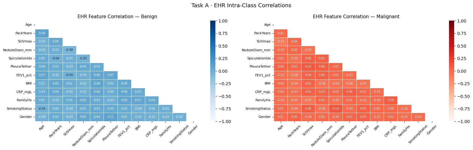
# ── 6.1e  Per-feature violin plots ──────────────────────────────────────────
plot_feats = ["Age", "PackYears", "SUVmax", "NoduleDiam_mm",
              "SpiculationIdx", "FEV1_pct", "CRP_mgL", "BMI"]
fig, axes = plt.subplots(2, 4, figsize=(18, 7))

for ax, feat in zip(axes.ravel(), plot_feats):
    data_b = meta[meta.Label == 0][feat].values
    data_m = meta[meta.Label == 1][feat].values
    parts  = ax.violinplot([data_b, data_m], positions=[0, 1],
                            showmedians=True, showextrema=True)
    for pc, color in zip(parts["bodies"], ["#3498db", "#e74c3c"]):
        pc.set_facecolor(color)
        pc.set_alpha(0.65)
    ax.set_xticks([0, 1])
    ax.set_xticklabels(["Benign", "Malignant"], fontsize=9)
    ax.set_title(feat, fontsize=10, fontweight="bold")
    ax.set_ylabel("Value", fontsize=8)

plt.suptitle("Task A · EHR Feature Distributions (Benign vs Malignant)", fontsize=13)
plt.tight_layout()
plt.show()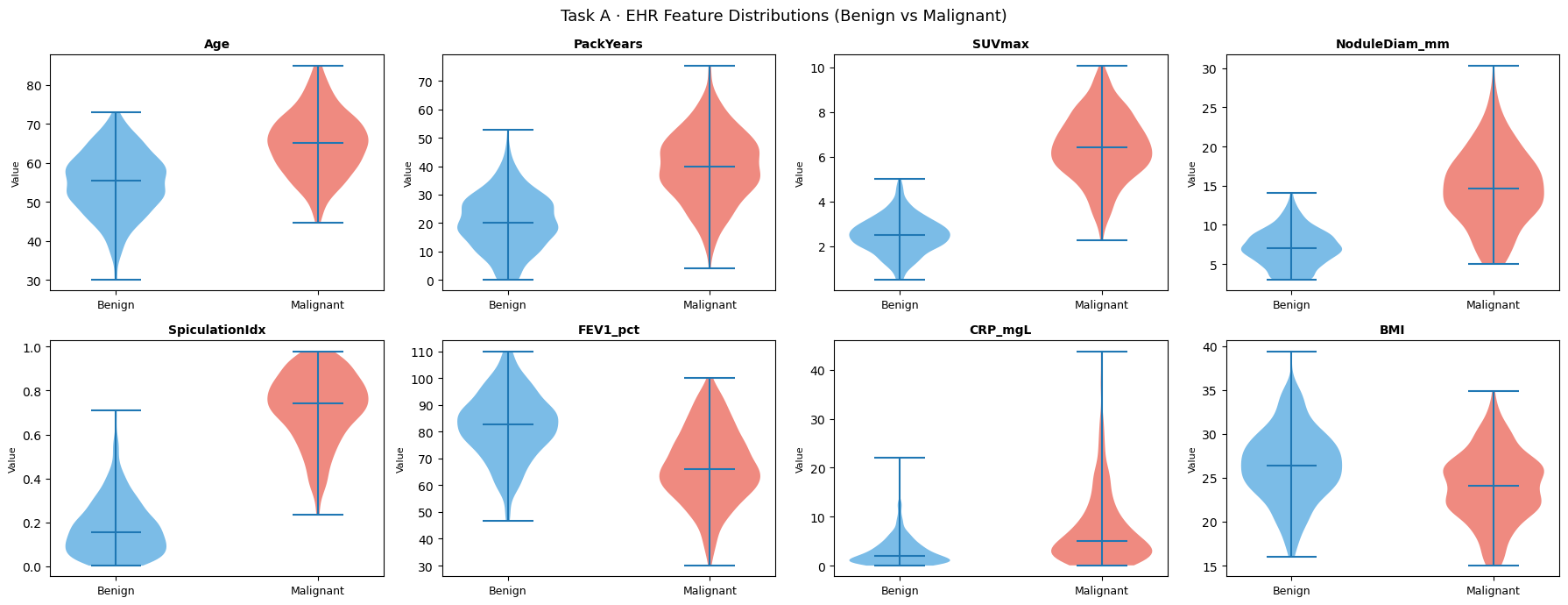
6.2 — Regression: T1 + T2 MRI (EDSS Score)
# ── 6.2a  Multi-score image montage ─────────────────────────────────────────
# Pick samples spanning the score range
sorted_idxs = np.argsort(reg_ds.scores)
pick_positions = np.linspace(0, len(sorted_idxs) - 1, 6, dtype=int)
pick_idxs = [sorted_idxs[p] for p in pick_positions]

fig, axes = plt.subplots(2, len(pick_idxs), figsize=(18, 6))

for col, idx in enumerate(pick_idxs):
    t1, t2, sc = reg_ds[idx]
    score = reg_ds.scores[idx]
    axes[0, col].imshow(t1.squeeze().numpy(), cmap="gray", vmin=0, vmax=1)
    axes[0, col].set_title(f"T1\nscore={score:.2f}", fontsize=9)
    axes[0, col].axis("off")
    axes[1, col].imshow(t2.squeeze().numpy(), cmap="gray", vmin=0, vmax=1)
    axes[1, col].set_title(f"T2\nscore={score:.2f}", fontsize=9)
    axes[1, col].axis("off")

plt.suptitle("Task B · T1 (top) & T2 (bottom) across EDSS-like score levels\n"
             "Expected: T1 periventricular hypointensities grow; T2 WMH burden increases",
             fontsize=11, y=1.02)
plt.tight_layout()
plt.show()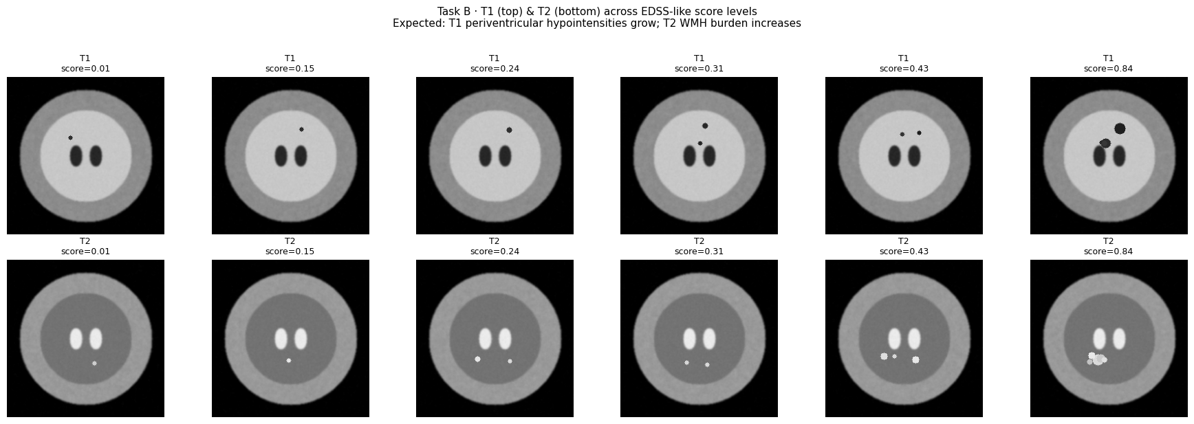
# ── 6.2b  Score distribution ────────────────────────────────────────────────
fig, axes = plt.subplots(1, 3, figsize=(15, 4))

scores_arr = np.array(reg_ds.scores)
axes[0].hist(scores_arr, bins=30, color="#2ecc71", edgecolor="white", linewidth=0.5)
axes[0].set_xlabel("EDSS-like score")
axes[0].set_ylabel("Count")
axes[0].set_title(f"Score Distribution\nMean={scores_arr.mean():.3f}  Std={scores_arr.std():.3f}")

# ── 6.2c  Mean T1/T2 intensity vs score (lesion area proxy) ─────────────────
n_probe = min(80, len(reg_ds))
probe_scores, mean_t1, mean_t2 = [], [], []
for i in range(n_probe):
    t1_img, t2_img, sc = reg_ds[i]
    probe_scores.append(sc.item())
    # Proxy: mean intensity in upper-central ROI (periventricular for T1)
    h, w = t1_img.shape[-2], t1_img.shape[-1]
    peri_t1 = t1_img[0, h//4: h//2, w//4: 3*w//4].mean().item()
    deep_t2 = t2_img[0, h//2: 3*h//4, w//4: 3*w//4].mean().item()
    mean_t1.append(peri_t1)
    mean_t2.append(deep_t2)

axes[1].scatter(probe_scores, mean_t1, alpha=0.55, s=18, color="#e74c3c", label="T1 periventr.")
z1 = np.polyfit(probe_scores, mean_t1, 1)
xs = np.linspace(0, 1, 50)
axes[1].plot(xs, np.polyval(z1, xs), color="#e74c3c", lw=2)
axes[1].set_xlabel("EDSS score"); axes[1].set_ylabel("ROI mean intensity")
axes[1].set_title("T1 Periventricular Intensity vs Score\n(expected: decreasing — T1 hypointensities)")
axes[1].legend()

axes[2].scatter(probe_scores, mean_t2, alpha=0.55, s=18, color="#3498db", label="T2 deep WM")
z2 = np.polyfit(probe_scores, mean_t2, 1)
axes[2].plot(xs, np.polyval(z2, xs), color="#3498db", lw=2)
axes[2].set_xlabel("EDSS score"); axes[2].set_ylabel("ROI mean intensity")
axes[2].set_title("T2 Deep WM Intensity vs Score\n(expected: increasing — WMH burden)")
axes[2].legend()

plt.tight_layout()
plt.show()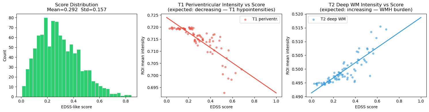
6.3 — Segmentation: FLAIR + T1ce (GBM-like Lesion)
# ── 6.3a  Multi-sample panel ─────────────────────────────────────────────────
n_show = 5
fig, axes = plt.subplots(4, n_show, figsize=(18, 12))
row_labels = ["FLAIR", "T1ce", "GT Mask", "Overlay"]

for col in range(n_show):
    flair, t1ce, mask = seg_ds[col]
    imgs = [flair.squeeze(), t1ce.squeeze(), mask.squeeze()]
    cmaps = ["gray", "gray", "Reds"]
    for row in range(3):
        axes[row, col].imshow(imgs[row].numpy(), cmap=cmaps[row], vmin=0, vmax=1)
        axes[row, col].axis("off")
        if col == 0:
            axes[row, col].set_ylabel(row_labels[row], fontsize=9, rotation=90,
                                       labelpad=4, fontweight="bold")
    # Overlay row
    axes[3, col].imshow(flair.squeeze().numpy(), cmap="gray", vmin=0, vmax=1)
    axes[3, col].imshow(mask.squeeze().numpy(), cmap="Reds", alpha=0.45, vmin=0, vmax=1)
    axes[3, col].axis("off")
    axes[3, col].set_title(f"Sample {col+1}", fontsize=9)
    if col == 0:
        axes[3, col].set_ylabel(row_labels[3], fontsize=9, rotation=90,
                                 labelpad=4, fontweight="bold")

plt.suptitle("Task C · FLAIR / T1ce / GT Mask / Overlay\n"
             "Note: ring-enhancing lesion (bright rim, dark core) + surrounding edema",
             fontsize=11, y=1.01)
plt.tight_layout()
plt.show()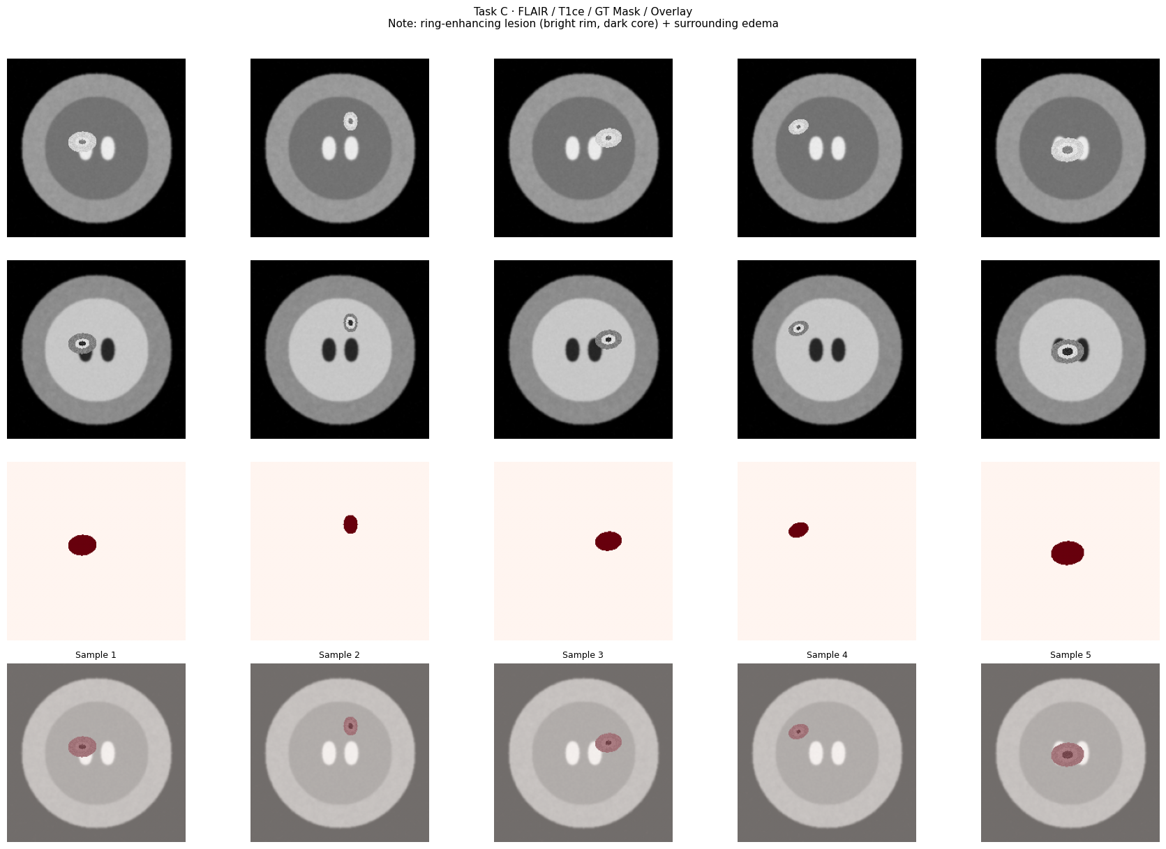
# ── 6.3b  Lesion statistics across dataset ──────────────────────────────────
n_stats = min(100, len(seg_ds))
lesion_sizes, flair_intensities, t1ce_ring_intensities = [], [], []

for i in range(n_stats):
    fl, t1, msk = seg_ds[i]
    msk_np = msk.squeeze().numpy()
    fl_np  = fl.squeeze().numpy()
    t1_np  = t1.squeeze().numpy()

    lesion_area = msk_np.sum()
    lesion_sizes.append(lesion_area)
    if lesion_area > 0:
        flair_intensities.append(fl_np[msk_np > 0.5].mean())
        # T1ce ring: pixels with high intensity inside mask
        t1ce_in_mask = t1_np[msk_np > 0.5]
        t1ce_ring_intensities.append(t1ce_in_mask[t1ce_in_mask > np.percentile(t1ce_in_mask, 60)].mean()
                                     if len(t1ce_in_mask) > 5 else np.nan)

fig, axes = plt.subplots(1, 3, figsize=(15, 4))

axes[0].hist(lesion_sizes, bins=25, color="#9b59b6", edgecolor="white", linewidth=0.5)
axes[0].set_xlabel("Lesion area (pixels)")
axes[0].set_ylabel("Count")
axes[0].set_title(f"GT Lesion Size Distribution\nMean={np.mean(lesion_sizes):.0f} px  "
                  f"Std={np.std(lesion_sizes):.0f} px")

axes[1].hist(flair_intensities, bins=25, color="#e67e22", edgecolor="white", linewidth=0.5)
axes[1].axvline(np.mean(flair_intensities), color="black", lw=1.5, linestyle="--",
                label=f"mean={np.mean(flair_intensities):.3f}")
axes[1].set_xlabel("Mean FLAIR intensity inside mask")
axes[1].set_title("FLAIR Lesion Intensity\n(expected: bright ≈ 0.80)")
axes[1].legend()

valid_ring = [v for v in t1ce_ring_intensities if not np.isnan(v)]
axes[2].hist(valid_ring, bins=25, color="#1abc9c", edgecolor="white", linewidth=0.5)
axes[2].axvline(np.mean(valid_ring), color="black", lw=1.5, linestyle="--",
                label=f"mean={np.mean(valid_ring):.3f}")
axes[2].set_xlabel("T1ce ring intensity (top 40% within mask)")
axes[2].set_title("T1ce Ring-Enhancement Intensity\n(expected: bright ≈ 0.85)")
axes[2].legend()

plt.suptitle("Task C · Lesion Statistics Across 100 Samples", fontsize=13)
plt.tight_layout()
plt.show()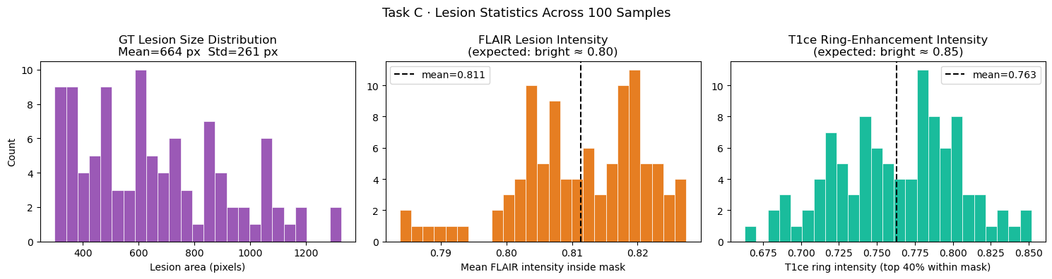
# ── 6.3c  Multi-compartment anatomy for one sample ──────────────────────────
# Use a specific sample from the dataset for detailed compartment analysis
flair_ex, t1ce_ex, mask_ex = seg_ds[42]

flair_np = flair_ex.squeeze().numpy()
t1ce_np  = t1ce_ex.squeeze().numpy()
mask_np  = mask_ex.squeeze().numpy()

# Build sub-compartment masks from intensity thresholds within GT mask
inside = mask_np > 0.5
if inside.sum() > 0:
    t1ce_inside = t1ce_np[inside]
    thresh_ring   = np.percentile(t1ce_inside, 60)
    thresh_necro  = np.percentile(t1ce_inside, 20)
    ring_px       = inside & (t1ce_np >= thresh_ring)
    necrosis_px   = inside & (t1ce_np <= thresh_necro)
    edema_px      = inside & ~ring_px & ~necrosis_px
else:
    ring_px = necrosis_px = edema_px = np.zeros_like(mask_np, dtype=bool)

# Color overlay: edema=yellow, ring=red, necrosis=blue
overlay = np.stack([flair_np, flair_np, flair_np], axis=-1)
overlay[edema_px]    = [0.90, 0.85, 0.10]   # yellow
overlay[ring_px]     = [0.90, 0.15, 0.15]   # red
overlay[necrosis_px] = [0.15, 0.35, 0.90]   # blue

fig, axes = plt.subplots(1, 5, figsize=(20, 4))
axes[0].imshow(flair_np,  cmap="gray");  axes[0].set_title("FLAIR");     axes[0].axis("off")
axes[1].imshow(t1ce_np,   cmap="gray");  axes[1].set_title("T1ce");      axes[1].axis("off")
axes[2].imshow(mask_np,   cmap="Reds");  axes[2].set_title("GT Mask");   axes[2].axis("off")
axes[3].imshow(overlay);                  axes[3].set_title("Compartments\nyellow=edema  red=rim  blue=necrosis")
axes[3].axis("off")

# Intensity profiles: horizontal line through lesion center
cy_les = int(np.where(mask_np.sum(axis=1) > 0)[0].mean()) if mask_np.sum() > 0 else IMG_SIZE // 2
axes[4].plot(flair_np[cy_les, :], color="#e67e22", label="FLAIR", lw=1.8)
axes[4].plot(t1ce_np[cy_les, :],  color="#3498db", label="T1ce",  lw=1.8)
axes[4].axhspan(0, 1, alpha=0.08, color="gray")
axes[4].fill_between(range(IMG_SIZE),
                      [0.0] * IMG_SIZE, [1.0] * IMG_SIZE,
                      where=mask_np[cy_les, :] > 0.5,
                      alpha=0.18, color="#e74c3c", label="Lesion region")
axes[4].set_xlabel("Pixel position (x)")
axes[4].set_ylabel("Normalised intensity")
axes[4].set_title(f"Intensity Profile — row {cy_les}")
axes[4].legend(fontsize=8)
axes[4].set_ylim(-0.05, 1.05)

plt.suptitle("Task C · Single-Sample Anatomy: Multi-compartment GBM-like Lesion",
             fontsize=12, y=1.02)
plt.tight_layout()
plt.show()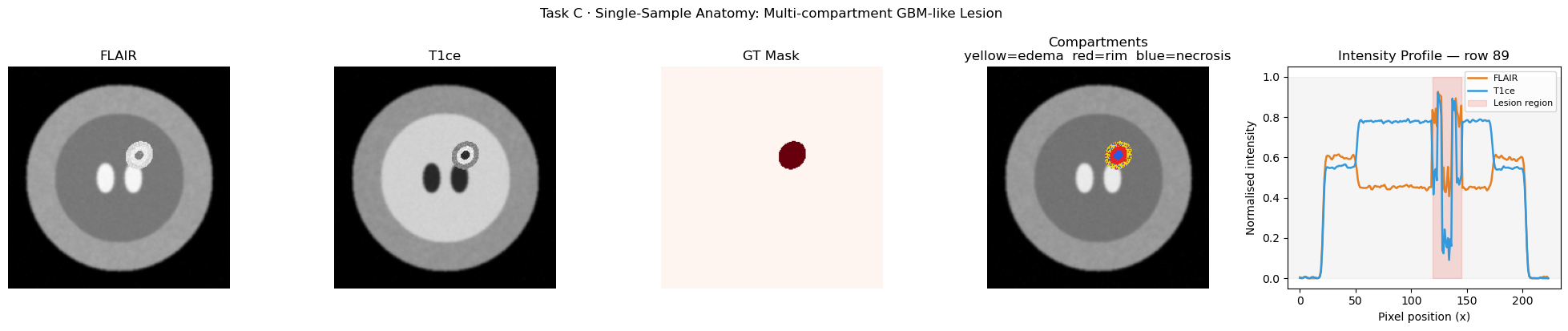
6.4 — Cross-Dataset Summary
fig, axes = plt.subplots(1, 3, figsize=(15, 5))

# ── Label balance (Classification) ──────────────────────────────────────────
label_counts = cls_ds.metadata["LabelName"].value_counts()
axes[0].bar(label_counts.index, label_counts.values,
             color=["#3498db", "#e74c3c"], alpha=0.85, edgecolor="white")
for i, (lbl, cnt) in enumerate(label_counts.items()):
    axes[0].text(i, cnt + 2, str(cnt), ha="center", fontsize=11, fontweight="bold")
axes[0].set_title("Task A · Class Balance")
axes[0].set_ylabel("Number of samples")
axes[0].set_ylim(0, label_counts.max() + 20)

# ── Score distribution (Regression) ─────────────────────────────────────────
axes[1].hist(reg_ds.scores, bins=30, color="#2ecc71", edgecolor="white", linewidth=0.5)
axes[1].set_xlabel("EDSS-like score (0=minimal, 1=severe)")
axes[1].set_ylabel("Count")
axes[1].set_title("Task B · Score Distribution\n(Beta(2,5) — skewed toward low disability)")

# ── Lesion area distribution (Segmentation) ──────────────────────────────────
n_eda = min(150, len(seg_ds))
areas = []
for i in range(n_eda):
    _, _, msk = seg_ds[i]
    areas.append(msk.squeeze().numpy().sum())
axes[2].hist(areas, bins=30, color="#9b59b6", edgecolor="white", linewidth=0.5)
axes[2].set_xlabel("Total lesion area (pixels)")
axes[2].set_ylabel("Count")
axes[2].set_title(f"Task C · GT Lesion Area Distribution\n(n={n_eda} samples)")

plt.suptitle("Cross-Dataset EDA Summary", fontsize=14, fontweight="bold")
plt.tight_layout()
plt.show()

# ── Print compact dataset card ───────────────────────────────────────────────
print("=" * 60)
print("DATASET CARD")
print("=" * 60)
print(f"Task A  CT + EHR Classification")
print(f"  Samples : {len(cls_ds)}  (50% benign / 50% malignant)")
print(f"  CT size : {IMG_SIZE}×{IMG_SIZE} px  |  EHR features: {len(EHR_FEATURE_NAMES)}")
print(f"  EHR mean (benign)   : age={cls_ds.metadata[cls_ds.metadata.Label==0]['Age'].mean():.1f}, "
      f"SUVmax={cls_ds.metadata[cls_ds.metadata.Label==0]['SUVmax'].mean():.2f}")
print(f"  EHR mean (malignant): age={cls_ds.metadata[cls_ds.metadata.Label==1]['Age'].mean():.1f}, "
      f"SUVmax={cls_ds.metadata[cls_ds.metadata.Label==1]['SUVmax'].mean():.2f}")
print()
print(f"Task B  T1+T2 MRI Regression")
print(f"  Samples : {len(reg_ds)}  |  Score: Beta(2,5)")
print(f"  Score stats: mean={np.mean(reg_ds.scores):.3f} ± {np.std(reg_ds.scores):.3f}  "
      f"[{np.min(reg_ds.scores):.3f}, {np.max(reg_ds.scores):.3f}]")
print()
print(f"Task C  FLAIR+T1ce Segmentation")
print(f"  Samples : {len(seg_ds)}")
print(f"  Lesion area: mean={np.mean(areas):.0f} ± {np.std(areas):.0f} px")
print("=" * 60)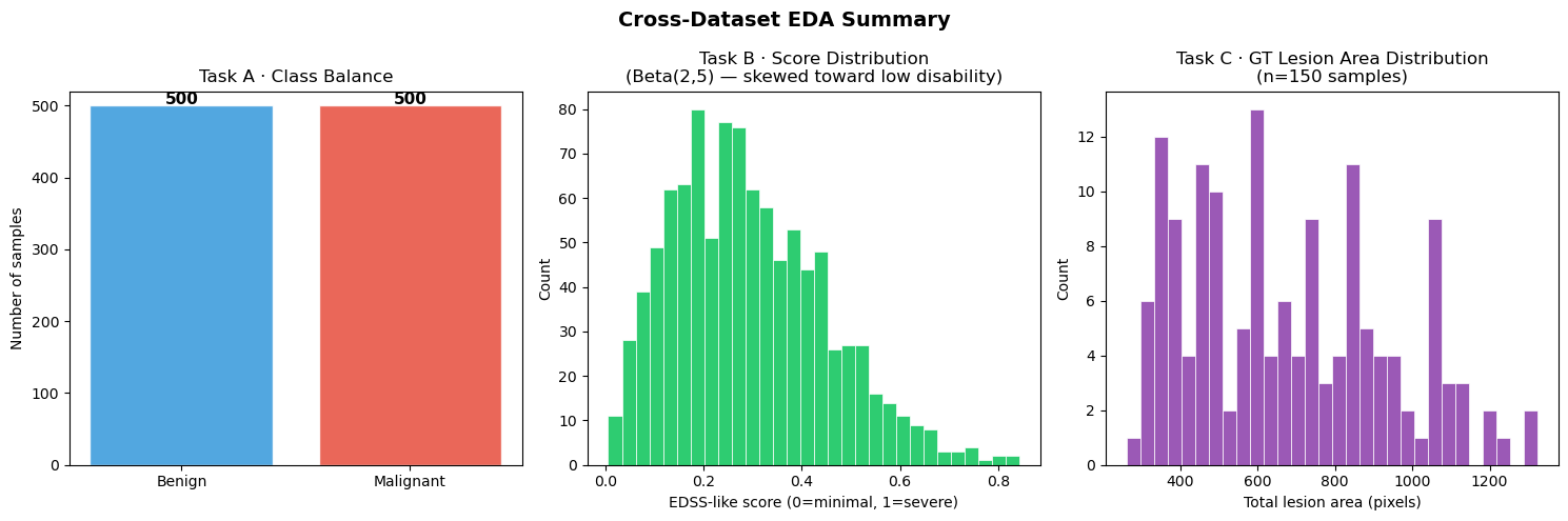
============================================================
DATASET CARD
============================================================
Task A  CT + EHR Classification
  Samples : 1000  (50% benign / 50% malignant)
  CT size : 224×224 px  |  EHR features: 12
  EHR mean (benign)   : age=54.9, SUVmax=2.50
  EHR mean (malignant): age=65.0, SUVmax=6.42

Task B  T1+T2 MRI Regression
  Samples : 1000  |  Score: Beta(2,5)
  Score stats: mean=0.292 ± 0.157  [0.006, 0.844]

Task C  FLAIR+T1ce Segmentation
  Samples : 1000
  Lesion area: mean=676 ± 260 px
============================================================
TASK A — Multi-Modal Classification (Image + Tabular)
Clinical analogy: Fusing a CT scan with structured EHR data to predict pathology presence.
Architecture
Image Stream: Conv(1→16)→ReLU→MaxPool → Conv(16→32)→ReLU→MaxPool → AdaptiveAvgPool → Linear(512→64)→ReLU
Tabular Stream: Linear(12→32)→ReLU → Linear(32→32)→ReLU
Fusion: cat[64+32] → Linear(96→64)→ReLU → Linear(64→2)
Architecture:
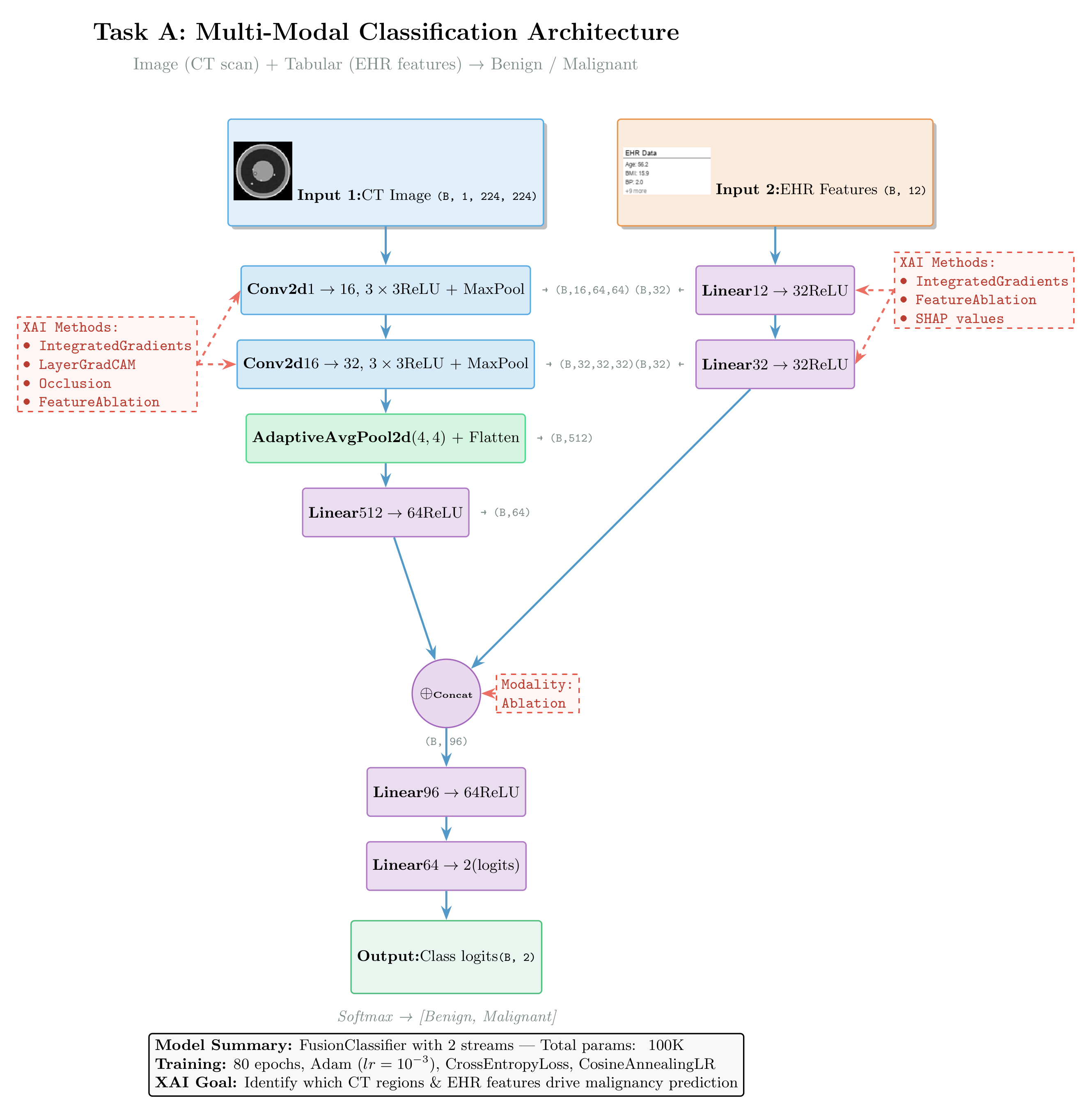
Figure: Multi-modal classification architecture fusing CT images (CNN) and electronic health records (MLP). The diagram shows which XAI methods apply to each component: Integrated Gradients and Saliency for feature attribution, GradCAM for convolutional layers, and Occlusion for perturbation-based analysis at the fusion level.
class FusionClassifier(nn.Module):
    def __init__(self, n_tabular=12):
        super().__init__()
        # Image stream — store as sequential for LayerGradCAM access
        self.image_encoder = nn.Sequential(
            nn.Conv2d(1, 16, 3, padding=1), nn.ReLU(), nn.MaxPool2d(2),  # 224→112
            nn.Conv2d(16, 32, 3, padding=1), nn.ReLU(), nn.MaxPool2d(2), # 112→56
        )
        self.img_head = nn.Sequential(
            nn.AdaptiveAvgPool2d((4, 4)),
            nn.Flatten(),
            nn.Linear(32 * 4 * 4, 64), nn.ReLU(),
        )
        # Tabular stream
        self.tab_encoder = nn.Sequential(
            nn.Linear(n_tabular, 32), nn.ReLU(),
            nn.Linear(32, 32),        nn.ReLU(),
        )
        # Fusion head
        self.fusion = nn.Sequential(
            nn.Linear(64 + 32, 64), nn.ReLU(),
            nn.Linear(64, 2),
        )

    def forward(self, image, tabular):
        img_feat = self.img_head(self.image_encoder(image))
        tab_feat = self.tab_encoder(tabular)
        return self.fusion(torch.cat([img_feat, tab_feat], dim=1))


cls_model = FusionClassifier(n_tabular=len(EHR_FEATURE_NAMES)).to(DEVICE)
print("FusionClassifier:", sum(p.numel() for p in cls_model.parameters()), "parameters")
FusionClassifier: 45442 parameters
# [PRE-RUN] Training loop — Classification
from pathlib import Path

cls_model_path = Path("cls_model.pt")
if cls_model_path.exists():
    print(f"✓ Found {cls_model_path} — loading pre-trained weights (skipping training)")
    cls_model.load_state_dict(torch.load(cls_model_path, map_location=DEVICE))
else:
    print("Training Classification model (80 epochs)...")
    optimizer = torch.optim.Adam(cls_model.parameters(), lr=1e-3)
    criterion = nn.CrossEntropyLoss()
    scheduler = torch.optim.lr_scheduler.CosineAnnealingLR(optimizer, T_max=80)

    cls_model.train()
    for epoch in range(80):
        total_loss, correct, total = 0.0, 0, 0
        for img, tab, label in cls_loader:
            img, tab, label = img.to(DEVICE), tab.to(DEVICE), label.to(DEVICE)
            optimizer.zero_grad()
            logits = cls_model(img, tab)
            loss = criterion(logits, label)
            loss.backward()
            optimizer.step()
            total_loss += loss.item() * len(label)
            correct += (logits.argmax(1) == label).sum().item()
            total += len(label)
        scheduler.step()
        if (epoch + 1) % 20 == 0:
            print(f"Epoch {epoch+1:3d} | loss={total_loss/total:.4f} | acc={correct/total:.1%} | lr={scheduler.get_last_lr()[0]:.5f}")

    torch.save(cls_model.state_dict(), "cls_model.pt")
    print("Saved cls_model.pt")
✓ Found cls_model.pt — loading pre-trained weights (skipping training)
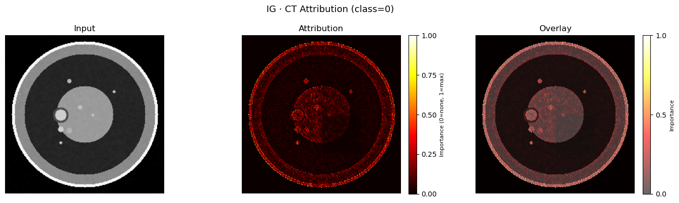
# [LIVE] Integrated Gradients — Classification (Image + Tabular)
cls_model.eval()
# Grab one sample
img_xai, tab_xai, label_xai = next(iter(cls_xai_loader))
img_xai = img_xai.to(DEVICE).requires_grad_(True)
tab_xai = tab_xai.to(DEVICE).requires_grad_(True)
with torch.no_grad():
pred_class = cls_model(img_xai, tab_xai).argmax(1).item()
ig = IntegratedGradients(cls_model)
attr_img_ig, attr_tab_ig = ig.attribute(
inputs=(img_xai, tab_xai),
baselines=(torch.zeros_like(img_xai), torch.zeros_like(tab_xai)),
target=pred_class,
n_steps=50,
return_convergence_delta=False,
)
print(f"Predicted class: {'Malignant' if pred_class==1 else 'Benign'}")
print(f"True label: {'Malignant' if label_xai.item()==1 else 'Benign'}")
# Spatial heatmap
plot_img_attr(img_xai, attr_img_ig, title=f"IG · CT Attribution (class={pred_class})")
plt.show()
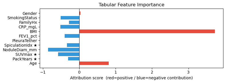
# Tabular bar chart — PackYears, SUVmax, SpiculationIdx marked ★ should dominate
# Mark clinically most discriminative features with ★
FEAT_NAMES = [
f"{n}" + (" ★" if n in ("PackYears", "SUVmax", "SpiculationIdx") else "")
for n in EHR_FEATURE_NAMES
]
plot_tabular_attr(attr_tab_ig, feature_names=FEAT_NAMES)
plt.show()Predicted class: Benign
True label: Benign
# [LIVE] DeepLIFT — Classification
dl = DeepLift(cls_model)
attr_img_dl, attr_tab_dl = dl.attribute(
inputs=(img_xai, tab_xai),
baselines=(torch.zeros_like(img_xai), torch.zeros_like(tab_xai)),
target=pred_class,
)
fig, axes = plt.subplots(1, 2, figsize=(10, 4))
axes[0].imshow(normalize_attr(attr_img_ig), cmap="hot"); axes[0].set_title("IG · Image"); axes[0].axis("off")
axes[1].imshow(normalize_attr(attr_img_dl), cmap="hot"); axes[1].set_title("DeepLIFT · Image"); axes[1].axis("off")
plt.suptitle("IG vs DeepLIFT — Spatial Attribution")
plt.tight_layout(); plt.show()
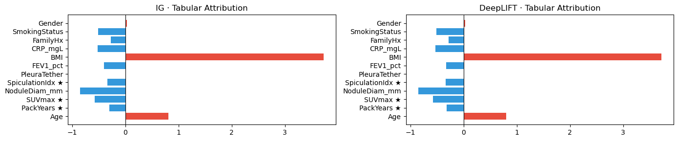
# Side-by-side tabular
fig, axes = plt.subplots(1, 2, figsize=(14, 3))
for ax, attr, name in zip(axes, [attr_tab_ig, attr_tab_dl], ["IG", "DeepLIFT"]):
vals = attr.squeeze().detach().cpu().numpy()
colors = ["#e74c3c" if v > 0 else "#3498db" for v in vals]
ax.barh(FEAT_NAMES, vals, color=colors)
ax.axvline(0, color="black", lw=0.8)
ax.set_title(f"{name} · Tabular Attribution")
plt.tight_layout(); plt.show()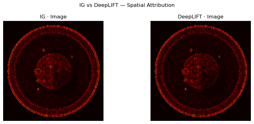
# [LIVE] GradientSHAP — Classification
gs = GradientShap(cls_model)
# Build stochastic baseline distribution (10 random samples per modality)
baseline_img_dist = torch.randn(10, *img_xai.shape[1:]).to(DEVICE)
baseline_tab_dist = torch.randn(10, *tab_xai.shape[1:]).to(DEVICE)

attr_img_gs, attr_tab_gs = gs.attribute(
    inputs=(img_xai, tab_xai),
    baselines=(baseline_img_dist, baseline_tab_dist),
    target=pred_class,
    n_samples=10,
    stdevs=0.1,
)

fig, axes = plt.subplots(1, 3, figsize=(15, 4))
for ax, attr, name in zip(axes, [attr_img_ig, attr_img_dl, attr_img_gs], ["IG", "DeepLIFT", "GradSHAP"]):
    ax.imshow(normalize_attr(attr), cmap="hot")
    ax.set_title(name); ax.axis("off")
plt.suptitle("Image Attribution Comparison (Classification)")
plt.tight_layout(); plt.show()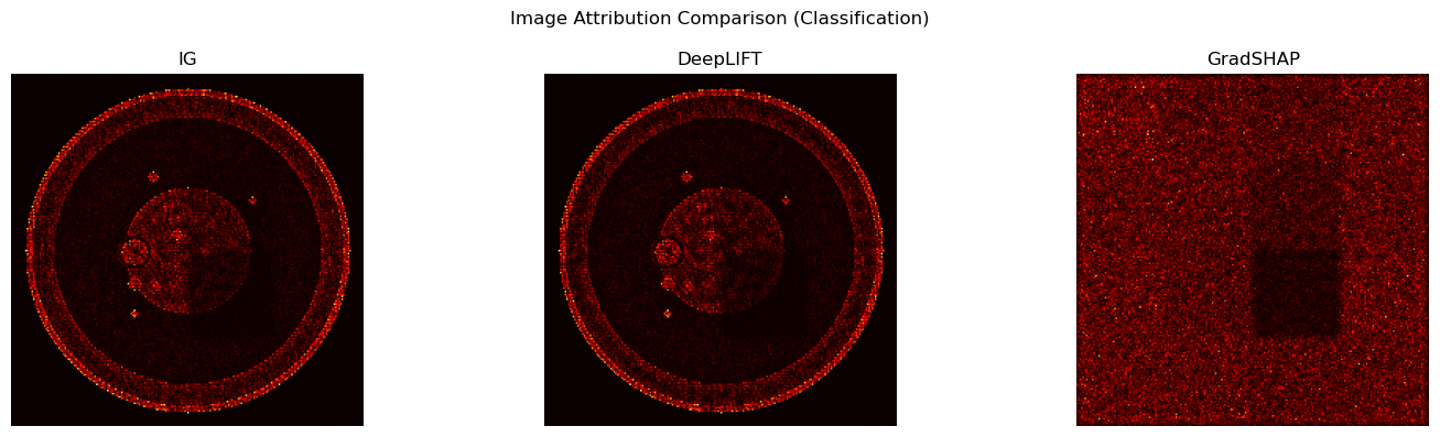
# [LIVE] LayerGradCAM — Image Stream Only
# GradCAM targets the last conv layer of the image encoder

# Wrapper that passes only image (tabular is fixed via closure)
class ImageOnlyWrapper(nn.Module):
    def __init__(self, model, tab):
        super().__init__()
        self.model = model
        self.tab = tab
    def forward(self, image):
        return self.model(image, self.tab)

img_only_model = ImageOnlyWrapper(cls_model, tab_xai).to(DEVICE)
target_layer = cls_model.image_encoder[-1]  # last Conv2d block

gcam = LayerGradCam(img_only_model, target_layer)
cam = gcam.attribute(img_xai, target=pred_class)
cam_upsampled = LayerAttribution.interpolate(cam, img_xai.shape[2:])

fig, axes = plt.subplots(1, 4, figsize=(16, 4))
for ax, attr, name in zip(axes, [attr_img_ig, attr_img_dl, attr_img_gs, cam_upsampled],
                           ["IG", "DeepLIFT", "GradSHAP", "GradCAM"]):
    ax.imshow(img_xai.squeeze().detach().cpu().numpy(), cmap="gray")
    ax.imshow(normalize_attr(attr), cmap="hot", alpha=0.5)
    ax.set_title(name); ax.axis("off")
plt.suptitle("2×2 Attribution Comparison — Classification (Overlay)")
plt.tight_layout(); plt.show()

print("Note: GradCAM only attributes the image stream. Pair with tabular IG for full picture.")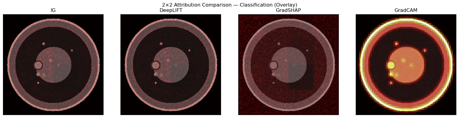
Note: GradCAM only attributes the image stream. Pair with tabular IG for full picture.
# [LIVE] Occlusion Sensitivity — Classification
cls_wrapper = MultiInputWrapper(cls_model)

occ = Occlusion(cls_wrapper)
attr_img_occ, attr_tab_occ = occ.attribute(
    inputs=(img_xai, tab_xai),
    sliding_window_shapes=((1, 8, 8), (1,)),
    target=pred_class,
    strides=((1, 4, 4), (1,)),
    baselines=(0.0, 0.0),
)

fig, axes = plt.subplots(1, 2, figsize=(10, 4))
axes[0].imshow(img_xai.squeeze().detach().cpu().numpy(), cmap="gray")
axes[0].imshow(normalize_attr(attr_img_occ), cmap="hot", alpha=0.5)
axes[0].set_title("Occlusion · Image"); axes[0].axis("off")

vals_occ = attr_tab_occ.squeeze().detach().cpu().numpy()
colors = ["#e74c3c" if v > 0 else "#3498db" for v in vals_occ]
axes[1].barh(FEAT_NAMES, vals_occ, color=colors)
axes[1].axvline(0, color="black", lw=0.8)
axes[1].set_title("Occlusion · Tabular")
plt.suptitle("Occlusion Sensitivity (Perturbation Baseline)")
plt.tight_layout(); plt.show()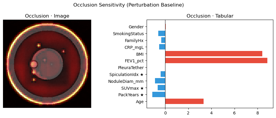
# [LIVE] Task A — XAI Gallery: Benign vs Malignant grid (IG attribution)
# Shows 4 benign and 4 malignant examples so class-specific patterns are visible.

cls_model.eval()
ig_gallery = IntegratedGradients(cls_model)

n_each = 4
benign_xai_idx  = [i for i in range(len(cls_xai_ds)) if int(cls_xai_ds.labels[i]) == 0][:n_each]
malig_xai_idx   = [i for i in range(len(cls_xai_ds)) if int(cls_xai_ds.labels[i]) == 1][:n_each]
all_gallery_idx = benign_xai_idx + malig_xai_idx
row_labels      = ["Benign"] * n_each + ["Malignant"] * n_each
border_colors   = ["#3498db"] * n_each + ["#e74c3c"] * n_each

fig, axes = plt.subplots(len(all_gallery_idx), 3, figsize=(13, 3 * len(all_gallery_idx)))
col_titles = ["CT Input", "IG Attribution", "Overlay (IG)"]
for col, ttl in enumerate(col_titles):
    axes[0, col].set_title(ttl, fontsize=11, fontweight="bold")

for row, (idx, lname, bcolor) in enumerate(zip(all_gallery_idx, row_labels, border_colors)):
    img_g, tab_g, lbl_g = cls_xai_ds[idx]
    img_g = img_g.unsqueeze(0).to(DEVICE).requires_grad_(True)
    tab_g = tab_g.unsqueeze(0).to(DEVICE).requires_grad_(True)

    with torch.no_grad():
        pred_g = cls_model(img_g, tab_g).argmax(1).item()

    attr_img_g, _ = ig_gallery.attribute(
        inputs=(img_g, tab_g),
        baselines=(torch.zeros_like(img_g), torch.zeros_like(tab_g)),
        target=pred_g, n_steps=50, return_convergence_delta=False,
    )
    img_np  = img_g.squeeze().detach().cpu().numpy()
    attr_np = normalize_attr(attr_img_g)
    pred_lbl = "Malignant" if pred_g == 1 else "Benign"
    true_lbl = "Malignant" if lbl_g.item() == 1 else "Benign"

    axes[row, 0].imshow(img_np, cmap="gray")
    axes[row, 0].axis("off")
    axes[row, 0].set_ylabel(f"{lname}\n(true={true_lbl}, pred={pred_lbl})",
                             fontsize=8, rotation=0, labelpad=90, va="center",
                             color=bcolor, fontweight="bold")
    for spine in axes[row, 0].spines.values():
        spine.set_edgecolor(bcolor); spine.set_linewidth(2)

    im_attr = axes[row, 1].imshow(attr_np, cmap="hot", vmin=0, vmax=1)
    axes[row, 1].axis("off")
    fig.colorbar(im_attr, ax=axes[row, 1], fraction=0.046, pad=0.04).set_label("Importance", fontsize=7)

    axes[row, 2].imshow(img_np, cmap="gray")
    im_ov = axes[row, 2].imshow(attr_np, cmap="hot", alpha=0.55, vmin=0, vmax=1)
    axes[row, 2].axis("off")
    fig.colorbar(im_ov, ax=axes[row, 2], fraction=0.046, pad=0.04).set_label("Importance", fontsize=7)

fig.suptitle(
    "Task A · IG Attribution Gallery — Top 4 Benign (blue) / Bottom 4 Malignant (red)\n"
    "Expected: malignant samples show nodule-region focus; benign samples show diffuse or absent signal",
    fontsize=12, y=1.01,
)
plt.tight_layout()
plt.show()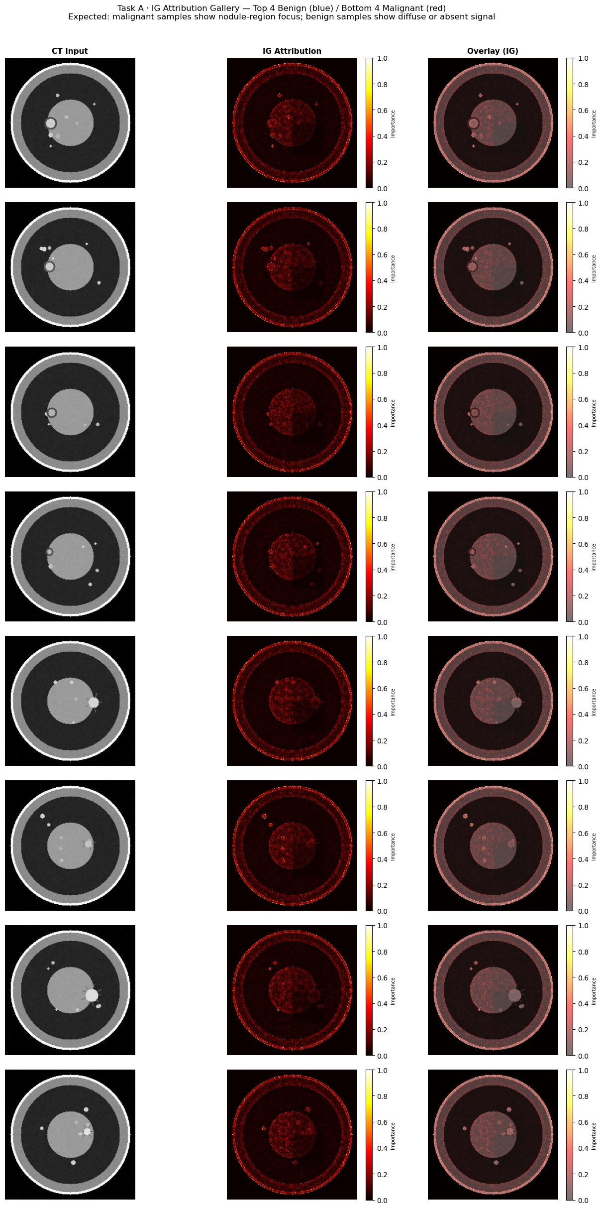
TASK B — Multi-Modal Regression (Image + Image)
Clinical analogy: Combining T1 and T2 MRI sequences to predict a continuous biomarker (e.g., tumor volume, EDSS score).
T1 top-left quadrant signal scales with score → IG should highlight top-left in T1
T2 bottom-right quadrant signal scales with score → IG should highlight bottom-right in T2
For regression, Captum uses target=0 to select the single scalar output neuron.
Architecture:
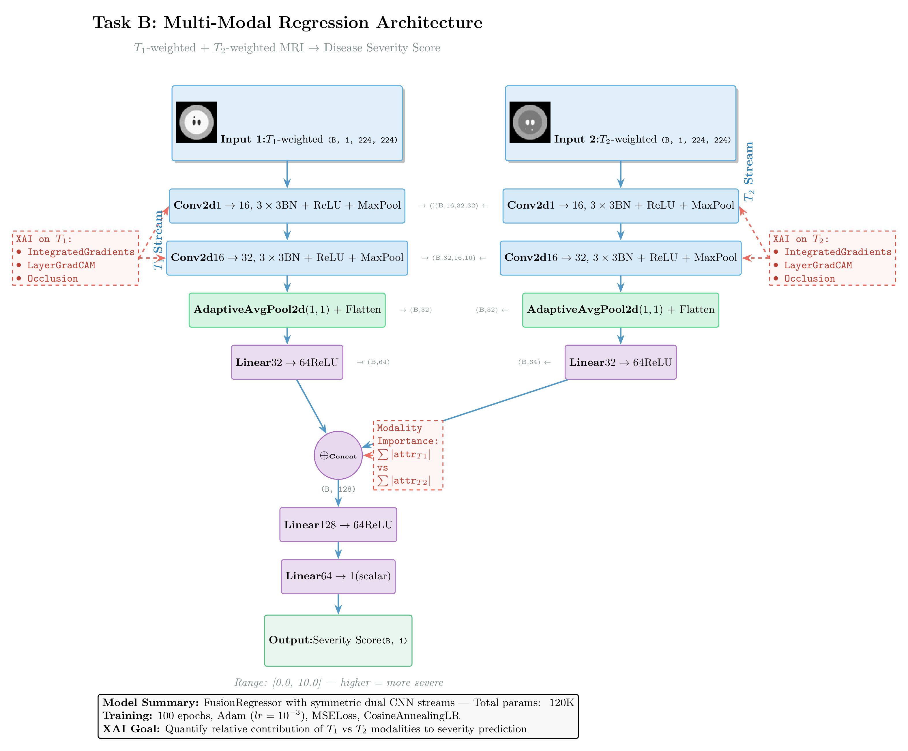
Figure: Dual-stream regression architecture fusing T1 and T2 MRI sequences to predict disease severity scores. Both encoders share identical CNN structure. The diagram annotates applicable XAI methods: Integrated Gradients and DeepLIFT for gradient-based attribution, and Feature Ablation for modality importance quantification.
class FusionRegressor(nn.Module):
    def __init__(self):
        super().__init__()
        def _stream():
            return nn.Sequential(
                nn.Conv2d(1, 16, 3, padding=1), nn.BatchNorm2d(16), nn.ReLU(), nn.MaxPool2d(2),
                nn.Conv2d(16, 32, 3, padding=1), nn.BatchNorm2d(32), nn.ReLU(), nn.MaxPool2d(2),
                nn.AdaptiveAvgPool2d((1, 1)), nn.Flatten(),
                nn.Linear(32, 64), nn.ReLU(),
            )

        self.t1_stream = _stream()
        self.t2_stream = _stream()
        self.fusion = nn.Sequential(
            nn.Linear(128, 64), nn.ReLU(),
            nn.Linear(64, 1),
        )

    def forward(self, t1, t2):
        return self.fusion(torch.cat([self.t1_stream(t1), self.t2_stream(t2)], dim=1))


reg_model = FusionRegressor().to(DEVICE)
print("FusionRegressor:", sum(p.numel() for p in reg_model.parameters()), "parameters")
FusionRegressor: 22337 parameters
# [PRE-RUN] Training loop — Regression
reg_model_path = Path("reg_model.pt")
if reg_model_path.exists():
    print(f"✓ Found {reg_model_path} — loading pre-trained weights (skipping training)")
    reg_model.load_state_dict(torch.load(reg_model_path, map_location=DEVICE))
else:
    print("Training Regression model (100 epochs)...")
    reg_optimizer = torch.optim.Adam(reg_model.parameters(), lr=1e-3)
    reg_criterion = nn.MSELoss()
    reg_scheduler = torch.optim.lr_scheduler.CosineAnnealingLR(reg_optimizer, T_max=100)

    reg_model.train()
    for epoch in range(100):
        total_loss, total = 0.0, 0
        for t1, t2, score in reg_loader:
            t1, t2, score = t1.to(DEVICE), t2.to(DEVICE), score.to(DEVICE)
            reg_optimizer.zero_grad()
            pred = reg_model(t1, t2)
            loss = reg_criterion(pred, score)
            loss.backward()
            reg_optimizer.step()
            total_loss += loss.item() * len(score)
            total += len(score)
        reg_scheduler.step()
        if (epoch + 1) % 20 == 0:
            rmse = (total_loss / total) ** 0.5
            print(f"Epoch {epoch+1:3d} | RMSE={rmse:.4f} | lr={reg_scheduler.get_last_lr()[0]:.5f}")

    torch.save(reg_model.state_dict(), "reg_model.pt")
    print("Saved reg_model.pt")
✓ Found reg_model.pt — loading pre-trained weights (skipping training)
# [LIVE] IG + Modality Importance — Regression
reg_model.eval()
t1_xai, t2_xai, score_xai = next(iter(reg_xai_loader))
t1_xai = t1_xai.to(DEVICE).requires_grad_(True)
t2_xai = t2_xai.to(DEVICE).requires_grad_(True)
ig_reg = IntegratedGradients(reg_model)
attr_t1, attr_t2 = ig_reg.attribute(
inputs=(t1_xai, t2_xai),
baselines=(torch.zeros_like(t1_xai), torch.zeros_like(t2_xai)),
target=0, # single scalar output → neuron index 0
n_steps=50,
)
# Verify spatial regions
fig, axes = plt.subplots(2, 3, figsize=(14, 8))
axes[0, 0].imshow(t1_xai.squeeze().detach().cpu().numpy(), cmap="gray")
axes[0, 0].set_title("T1 input"); axes[0, 0].axis("off")
axes[0, 1].imshow(normalize_attr(attr_t1), cmap="hot")
axes[0, 1].set_title("IG · T1 (expected: top-left)"); axes[0, 1].axis("off")
axes[0, 2].imshow(t1_xai.squeeze().detach().cpu().numpy(), cmap="gray")
axes[0, 2].imshow(normalize_attr(attr_t1), cmap="hot", alpha=0.5)
axes[0, 2].set_title("T1 overlay"); axes[0, 2].axis("off")
axes[1, 0].imshow(t2_xai.squeeze().detach().cpu().numpy(), cmap="gray")
axes[1, 0].set_title("T2 input"); axes[1, 0].axis("off")
axes[1, 1].imshow(normalize_attr(attr_t2), cmap="hot")
axes[1, 1].set_title("IG · T2 (expected: bottom-right)"); axes[1, 1].axis("off")
axes[1, 2].imshow(t2_xai.squeeze().detach().cpu().numpy(), cmap="gray")
axes[1, 2].imshow(normalize_attr(attr_t2), cmap="hot", alpha=0.5)
axes[1, 2].set_title("T2 overlay"); axes[1, 2].axis("off")
plt.suptitle(f"IG Regression (score={score_xai.item():.3f})")
plt.tight_layout(); plt.show()
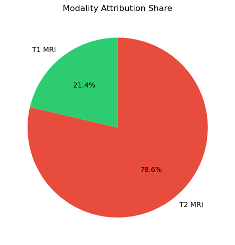
# Modality importance
imp_t1 = attr_t1.abs().mean().item()
imp_t2 = attr_t2.abs().mean().item()
total_imp = imp_t1 + imp_t2
print(f"T1 contribution: {imp_t1/total_imp:.1%} | T2 contribution: {imp_t2/total_imp:.1%}")
plot_modality_importance({"T1 MRI": imp_t1, "T2 MRI": imp_t2})
plt.show()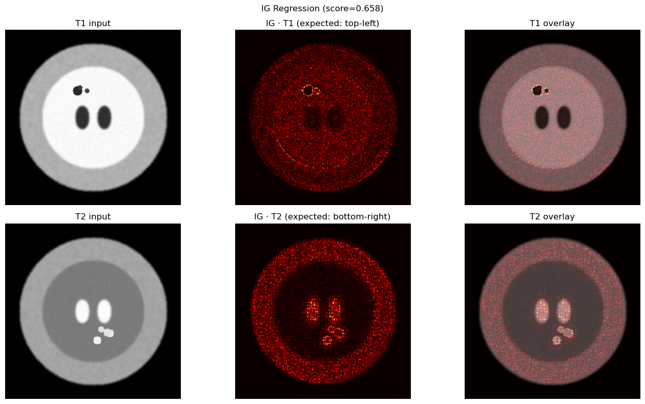
T1 contribution: 21.4% | T2 contribution: 78.6%
# [LIVE] DeepLIFT & Saliency comparison — Regression
dl_reg  = DeepLift(reg_model)
sal_reg = Saliency(reg_model)

attr_t1_dl, attr_t2_dl = dl_reg.attribute(
    inputs=(t1_xai, t2_xai),
    baselines=(torch.zeros_like(t1_xai), torch.zeros_like(t2_xai)),
    target=0,
)
attr_t1_sal, attr_t2_sal = sal_reg.attribute(
    inputs=(t1_xai, t2_xai),
    target=0,
    abs=False,
)

methods = ["IG", "DeepLIFT", "Saliency"]
attrs_t1 = [attr_t1, attr_t1_dl, attr_t1_sal]
attrs_t2 = [attr_t2, attr_t2_dl, attr_t2_sal]

fig, axes = plt.subplots(2, 3, figsize=(14, 8))
for col, (name, a1, a2) in enumerate(zip(methods, attrs_t1, attrs_t2)):
    axes[0, col].imshow(normalize_attr(a1), cmap="hot")
    axes[0, col].set_title(f"{name} · T1"); axes[0, col].axis("off")
    axes[1, col].imshow(normalize_attr(a2), cmap="hot")
    axes[1, col].set_title(f"{name} · T2"); axes[1, col].axis("off")
plt.suptitle("IG / DeepLIFT / Saliency — T1 (top) vs T2 (bottom)")
plt.tight_layout(); plt.show()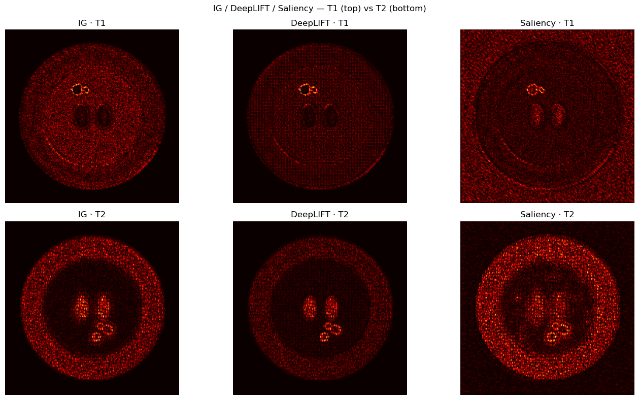
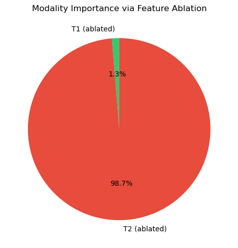
# [LIVE] Feature Ablation — Modality-Level Importance
reg_wrapper = MultiInputWrapper(reg_model)
fa = FeatureAblation(reg_wrapper)

# Assign all T1 pixels to group 1, all T2 pixels to group 2
mask_t1 = torch.ones_like(t1_xai, dtype=torch.long)          # group 1
mask_t2 = torch.ones_like(t2_xai, dtype=torch.long) * 2      # group 2

fa_attr_t1, fa_attr_t2 = fa.attribute(
    inputs=(t1_xai, t2_xai),
    feature_mask=(mask_t1, mask_t2),
    baselines=(torch.zeros_like(t1_xai), torch.zeros_like(t2_xai)),
    target=0,
)

with torch.no_grad():
    full_pred  = reg_model(t1_xai, t2_xai).item()
    zero_t1    = reg_model(torch.zeros_like(t1_xai), t2_xai).item()
    zero_t2    = reg_model(t1_xai, torch.zeros_like(t2_xai)).item()

print(f"Full prediction:    {full_pred:.4f}")
print(f"Ablate T1 → zero:  {zero_t1:.4f}  (drop: {full_pred - zero_t1:+.4f})")
print(f"Ablate T2 → zero:  {zero_t2:.4f}  (drop: {full_pred - zero_t2:+.4f})")

# Modality importance via ablation
drop_t1 = abs(full_pred - zero_t1)
drop_t2 = abs(full_pred - zero_t2)
plot_modality_importance({"T1 (ablated)": drop_t1, "T2 (ablated)": drop_t2},
                         title="Modality Importance via Feature Ablation")
plt.show()
Full prediction: 0.5219
Ablate T1 → zero: 0.5134 (drop: +0.0085)
Ablate T2 → zero: -0.1432 (drop: +0.6651)
# [LIVE] Task B — XAI Gallery: IG across score spectrum
# Pick 6 samples spanning low→high EDSS-like scores and show T1/T2 IG attributions.

reg_model.eval()
ig_reg_gallery = IntegratedGradients(reg_model)

# Sort XAI subset by predicted score and pick 6 evenly spaced samples
reg_xai_scores_list = []
for i in range(len(reg_xai_ds)):
    t1_tmp, t2_tmp, sc_tmp = reg_xai_ds[i]
    reg_xai_scores_list.append((i, sc_tmp.item()))

reg_xai_scores_list.sort(key=lambda x: x[1])
pick_pos    = np.linspace(0, len(reg_xai_scores_list) - 1, 6, dtype=int)
gallery_reg = [reg_xai_scores_list[p] for p in pick_pos]

fig, axes = plt.subplots(6, 6, figsize=(22, 22))
col_titles = ["T1 Input", "T1 IG", "T1 Overlay", "T2 Input", "T2 IG", "T2 Overlay"]
for col, ttl in enumerate(col_titles):
    axes[0, col].set_title(ttl, fontsize=10, fontweight="bold")

for row, (idx, score_val) in enumerate(gallery_reg):
    t1_g, t2_g, sc_g = reg_xai_ds[idx]
    t1_g = t1_g.unsqueeze(0).to(DEVICE).requires_grad_(True)
    t2_g = t2_g.unsqueeze(0).to(DEVICE).requires_grad_(True)

    attr_t1_g, attr_t2_g = ig_reg_gallery.attribute(
        inputs=(t1_g, t2_g),
        baselines=(torch.zeros_like(t1_g), torch.zeros_like(t2_g)),
        target=0, n_steps=50,
    )

    t1_np   = t1_g.squeeze().detach().cpu().numpy()
    t2_np   = t2_g.squeeze().detach().cpu().numpy()
    attr_t1 = normalize_attr(attr_t1_g)
    attr_t2 = normalize_attr(attr_t2_g)

    # T1 columns
    axes[row, 0].imshow(t1_np, cmap="gray"); axes[row, 0].axis("off")
    im1 = axes[row, 1].imshow(attr_t1, cmap="hot", vmin=0, vmax=1); axes[row, 1].axis("off")
    fig.colorbar(im1, ax=axes[row, 1], fraction=0.046, pad=0.04).set_label("Imp.", fontsize=6)
    axes[row, 2].imshow(t1_np, cmap="gray")
    im12 = axes[row, 2].imshow(attr_t1, cmap="hot", alpha=0.55, vmin=0, vmax=1); axes[row, 2].axis("off")
    fig.colorbar(im12, ax=axes[row, 2], fraction=0.046, pad=0.04).set_label("Imp.", fontsize=6)

    # T2 columns
    axes[row, 3].imshow(t2_np, cmap="gray"); axes[row, 3].axis("off")
    im2 = axes[row, 4].imshow(attr_t2, cmap="hot", vmin=0, vmax=1); axes[row, 4].axis("off")
    fig.colorbar(im2, ax=axes[row, 4], fraction=0.046, pad=0.04).set_label("Imp.", fontsize=6)
    axes[row, 5].imshow(t2_np, cmap="gray")
    im22 = axes[row, 5].imshow(attr_t2, cmap="hot", alpha=0.55, vmin=0, vmax=1); axes[row, 5].axis("off")
    fig.colorbar(im22, ax=axes[row, 5], fraction=0.046, pad=0.04).set_label("Imp.", fontsize=6)

    axes[row, 0].set_ylabel(f"score={score_val:.3f}", fontsize=9, rotation=0, labelpad=68, va="center")

fig.suptitle(
    "Task B · IG Gallery — T1 (cols 1–3) and T2 (cols 4–6) across EDSS-like score range\n"
    "Expected: low scores → sparse attribution; high scores → T1 top-left + T2 bottom-right focus",
    fontsize=12, y=1.01,
)
plt.tight_layout()
plt.show()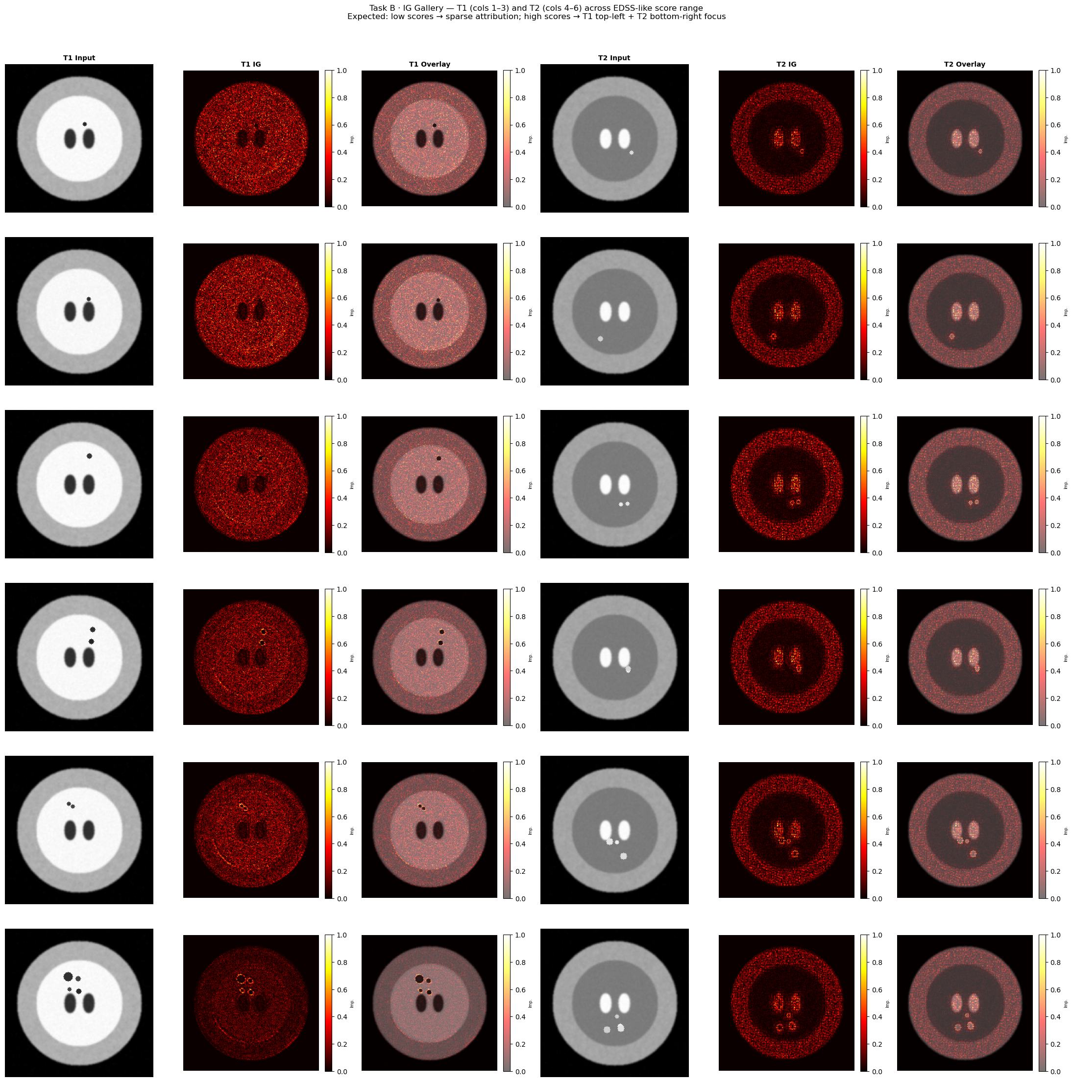
TASK C — Multi-Modal Segmentation (Image + Image → Pixel Mask)
Clinical analogy: Using FLAIR + T1ce sequences to segment brain tumor lesions (BraTS-inspired).
Key XAI challenge for segmentation: Captum needs a scalar output. We use SegReductionWrapper to collapse (B, 1, H, W) → (B, 1) via spatial mean, enabling gradient flow through a single target neuron.
Expected result: IG attribution for FLAIR should concentrate on the bright elliptical lesion region; T1ce attribution should show the same lesion at lower intensity.
Architecture:
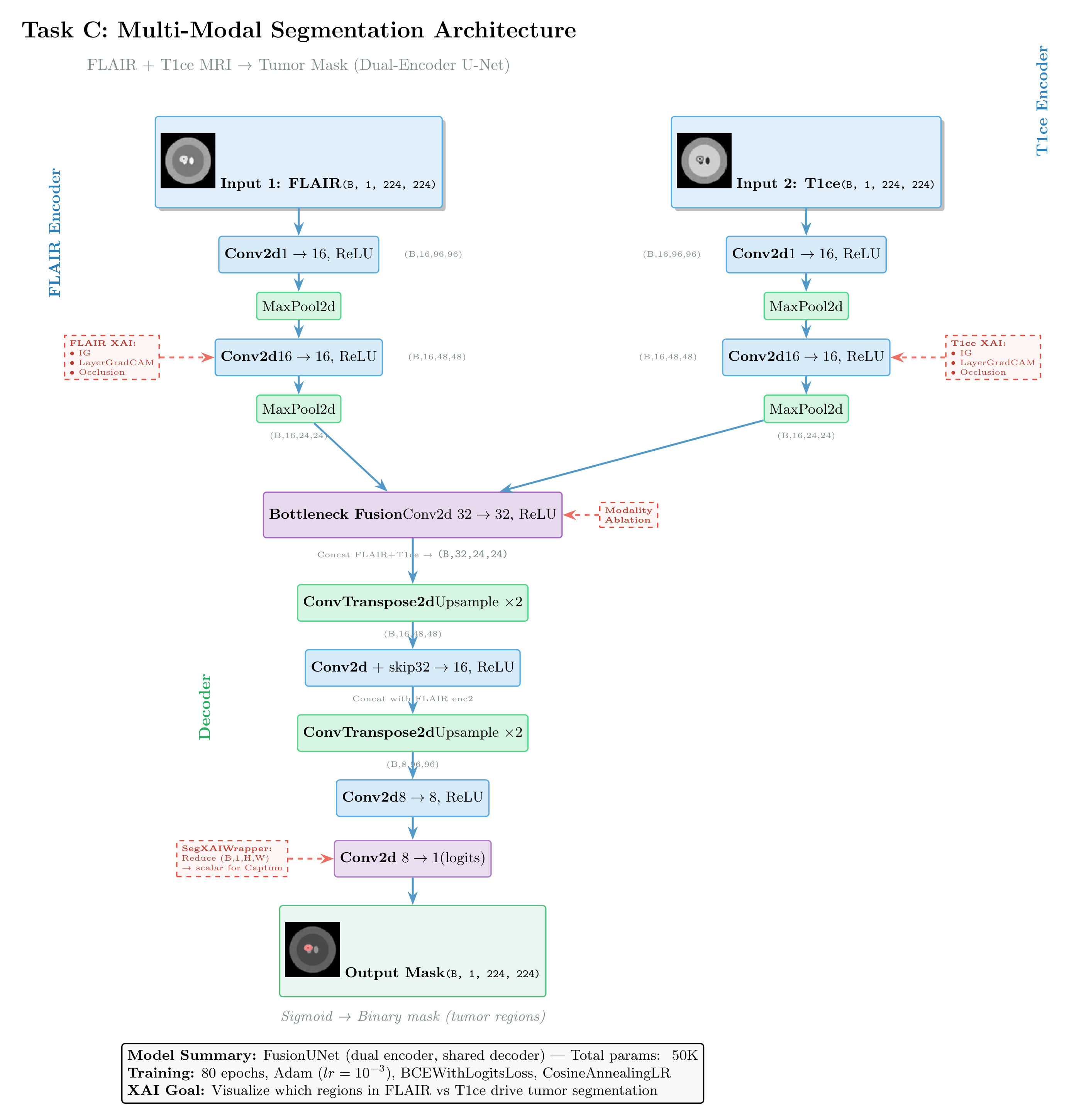
Figure: Dual-encoder U-Net architecture for multi-modal segmentation, fusing FLAIR and T1ce MRI sequences. Features from both encoders merge at the bottleneck, then decode with skip connections from the FLAIR pathway. The diagram shows applicable XAI methods: GradCAM for branch-specific feature visualization, and Integrated Gradients (via SegReductionWrapper) for pixel-level attribution.
class FusionUNet(nn.Module):
    """Lightweight dual-encoder U-Net for two-modality segmentation."""

    def __init__(self):
        super().__init__()
        # FLAIR encoder
        self.flair_enc1 = nn.Sequential(nn.Conv2d(1, 16, 3, padding=1), nn.ReLU())
        self.flair_pool1 = nn.MaxPool2d(2)
        self.flair_enc2 = nn.Sequential(nn.Conv2d(16, 16, 3, padding=1), nn.ReLU())
        self.flair_pool2 = nn.MaxPool2d(2)
        self.flair_last_conv = self.flair_enc2  # reference for GradCAM

        # T1ce encoder (identical structure)
        self.t1ce_enc1 = nn.Sequential(nn.Conv2d(1, 16, 3, padding=1), nn.ReLU())
        self.t1ce_pool1 = nn.MaxPool2d(2)
        self.t1ce_enc2 = nn.Sequential(nn.Conv2d(16, 16, 3, padding=1), nn.ReLU())
        self.t1ce_pool2 = nn.MaxPool2d(2)
        self.t1ce_last_conv = self.t1ce_enc2  # reference for GradCAM

        # Bottleneck fusion
        self.bottleneck = nn.Sequential(nn.Conv2d(32, 32, 3, padding=1), nn.ReLU())

        # Decoder
        self.up1 = nn.ConvTranspose2d(32, 16, 2, stride=2)
        self.dec1 = nn.Sequential(nn.Conv2d(32, 16, 3, padding=1), nn.ReLU())  # skip from flair_enc1
        self.up2 = nn.ConvTranspose2d(16, 8, 2, stride=2)
        self.dec2 = nn.Sequential(nn.Conv2d(8, 8, 3, padding=1), nn.ReLU())
        self.out_conv = nn.Conv2d(8, 1, 1)   # logits (no sigmoid — use BCEWithLogitsLoss)

    def forward(self, flair, t1ce):
        # FLAIR branch
        f1 = self.flair_enc1(flair)
        f2 = self.flair_enc2(self.flair_pool1(f1))
        fb = self.flair_pool2(f2)

        # T1ce branch
        t1 = self.t1ce_enc1(t1ce)
        t2 = self.t1ce_enc2(self.t1ce_pool1(t1))
        tb = self.t1ce_pool2(t2)

        # Fusion at bottleneck
        x = self.bottleneck(torch.cat([fb, tb], dim=1))

        # Decoder with skip from flair encoder level 1
        x = self.up1(x)
        x = self.dec1(torch.cat([x, f2], dim=1))
        x = self.up2(x)
        x = self.dec2(x)
        return self.out_conv(x)   # (B, 1, H, W) logits

seg_model = FusionUNet()

seg_model_path = Path("seg_model.pt")
if seg_model_path.exists():
    print(f"✓ Found {seg_model_path} — loading pre-trained weights (skipping training)")
    seg_model.load_state_dict(torch.load(seg_model_path, map_location=DEVICE))
else:
    print("Training Segmentation model (80 epochs)...")
    seg_optimizer = torch.optim.Adam(seg_model.parameters(), lr=1e-3)
    seg_criterion = nn.BCEWithLogitsLoss()
    seg_scheduler = torch.optim.lr_scheduler.CosineAnnealingLR(seg_optimizer, T_max=80)

    seg_model.train()
    for epoch in range(80):
        total_loss, total = 0.0, 0
        for flair_b, t1ce_b, mask_b in seg_loader:
            flair_b, t1ce_b, mask_b = flair_b.to(DEVICE), t1ce_b.to(DEVICE), mask_b.to(DEVICE)
            seg_optimizer.zero_grad()
            logits = seg_model(flair_b, t1ce_b)
            loss = seg_criterion(logits, mask_b)
            loss.backward()
            seg_optimizer.step()
            total_loss += loss.item() * len(mask_b)
            total += len(mask_b)
        seg_scheduler.step()
        if (epoch + 1) % 20 == 0:
            print(f"Epoch {epoch+1:3d} | loss={total_loss/total:.4f} | lr={seg_scheduler.get_last_lr()[0]:.5f}")

    # Dice coefficient on training set
    seg_model.eval()
    dice_scores = []
    with torch.no_grad():
        for flair_b, t1ce_b, mask_b in seg_loader:
            flair_b, t1ce_b, mask_b = flair_b.to(DEVICE), t1ce_b.to(DEVICE), mask_b.to(DEVICE)
            pred = torch.sigmoid(seg_model(flair_b, t1ce_b)) > 0.5
            intersection = (pred * mask_b.bool()).sum().float()
            dice = 2 * intersection / (pred.sum() + mask_b.sum() + 1e-8)
            dice_scores.append(dice.item())
    print(f"Mean Dice: {np.mean(dice_scores):.4f}")

    torch.save(seg_model.state_dict(), "seg_model.pt")
    intersection = (pred * mask_b.bool()).sum().float()
    dice = 2 * intersection / (pred.sum() + mask_b.sum() + 1e-8)
    dice_scores.append(dice.item())
    print(f"Mean Dice: {np.mean(dice_scores):.4f}")

    torch.save(seg_model.state_dict(), "seg_model.pt")
    print("Saved seg_model.pt")
✓ Found seg_model.pt — loading pre-trained weights (skipping training)
# SegXAIWrapper & lesion centroid helper
class SegXAIWrapper(nn.Module):
    """Reduces (B,1,H,W) segmentation output to (B,1) scalar for Captum."""
    def __init__(self, model, reduction="mean"):
        super().__init__()
        self.model = model
        self.reduction = reduction

    def forward(self, flair, t1ce):
        out = torch.sigmoid(self.model(flair, t1ce))   # (B, 1, H, W)
        if self.reduction == "mean":
            return out.mean(dim=(2, 3))                # (B, 1)
        return out.sum(dim=(2, 3))


def get_lesion_centroid(pred_mask):
    """Return (row, col) centroid of predicted lesion, or None if empty."""
    coords = pred_mask.squeeze().nonzero(as_tuple=False).float()
    if len(coords) == 0:
        return None
    return coords.mean(0).long().tolist()


seg_xai_model = SegXAIWrapper(seg_model).to(DEVICE)
print("SegXAIWrapper and centroid helper ready.")
SegXAIWrapper and centroid helper ready.
# [LIVE] IG — Segmentation (spatial attribution per modality)
seg_model.eval()

flair_xai, t1ce_xai, mask_xai = next(iter(seg_xai_loader))
flair_xai = flair_xai.to(DEVICE).requires_grad_(True)
t1ce_xai  = t1ce_xai.to(DEVICE).requires_grad_(True)

ig_seg = IntegratedGradients(seg_xai_model)
attr_flair, attr_t1ce = ig_seg.attribute(
    inputs=(flair_xai, t1ce_xai),
    baselines=(torch.zeros_like(flair_xai), torch.zeros_like(t1ce_xai)),
    target=0,
    n_steps=50,
)

# Predicted mask
with torch.no_grad():
    pred_mask = (torch.sigmoid(seg_model(flair_xai, t1ce_xai)) > 0.5).float()

centroid = get_lesion_centroid(pred_mask)
print(f"Predicted lesion centroid: {centroid}")
print(f"FLAIR attr max region: {normalize_attr(attr_flair).argmax()}")

# Modality importance for segmentation
imp_flair = attr_flair.abs().mean().item()
imp_t1ce  = attr_t1ce.abs().mean().item()
total_seg = imp_flair + imp_t1ce
print(f"FLAIR contribution: {imp_flair/total_seg:.1%}  |  T1ce contribution: {imp_t1ce/total_seg:.1%}")
Predicted lesion centroid: [121, 81]
FLAIR attr max region: 27629
FLAIR contribution: 25.7% | T1ce contribution: 74.3%
# [LIVE] LayerGradCAM — Dual Encoder (FLAIR + T1ce branches)
#
# seg_model outputs (B, 1, H, W) — LayerGradCam needs a scalar target.
# We pass seg_xai_model (SegReductionWrapper → output=(B,1)) and target=0.

# FLAIR encoder GradCAM — pass t1ce as additional arg
gcam_flair = LayerGradCam(seg_xai_model, seg_model.flair_last_conv)
cam_flair = gcam_flair.attribute(flair_xai, additional_forward_args=(t1ce_xai,), target=0)
cam_flair_up = LayerAttribution.interpolate(cam_flair, flair_xai.shape[2:])

# T1ce encoder GradCAM — pass flair as additional arg
gcam_t1ce = LayerGradCam(seg_xai_model, seg_model.t1ce_last_conv)
cam_t1ce = gcam_t1ce.attribute(t1ce_xai, additional_forward_args=(flair_xai,), target=0)
cam_t1ce_up = LayerAttribution.interpolate(cam_t1ce, t1ce_xai.shape[2:])

fig, axes = plt.subplots(1, 4, figsize=(16, 4))
ims = [flair_xai, t1ce_xai, cam_flair_up, cam_t1ce_up]
titles = ["FLAIR input", "T1ce input", "GradCAM · FLAIR enc", "GradCAM · T1ce enc"]
for ax, im, title in zip(axes, ims, titles):
    base = im.squeeze().detach().cpu().abs().numpy()
    ax.imshow(base, cmap="hot"); ax.set_title(title); ax.axis("off")
plt.suptitle("LayerGradCAM — Dual Encoder Attribution")
plt.tight_layout(); plt.show()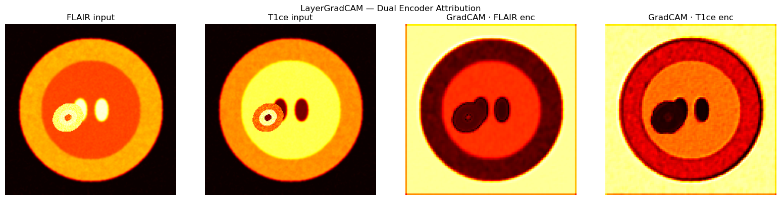
# [LIVE] Positive/Negative Attribution Decomposition

pos_attr_flair = torch.clamp(attr_flair, min=0)
neg_attr_flair = torch.clamp(attr_flair, max=0).abs()

fig, axes = plt.subplots(1, 4, figsize=(16, 4))
axes[0].imshow(flair_xai.squeeze().detach().cpu().numpy(), cmap="gray")
axes[0].set_title("FLAIR input"); axes[0].axis("off")

axes[1].imshow(normalize_attr(pos_attr_flair), cmap="Reds")
axes[1].set_title("Positive attr (FOR lesion)"); axes[1].axis("off")

axes[2].imshow(normalize_attr(neg_attr_flair), cmap="Blues")
axes[2].set_title("Negative attr (AGAINST lesion)"); axes[2].axis("off")

# Combined: RdBu diverging
combined = attr_flair.squeeze().detach().cpu().numpy()
vmax = np.abs(combined).max()
axes[3].imshow(combined, cmap="RdBu", vmin=-vmax, vmax=vmax)
axes[3].set_title("Combined (RdBu)"); axes[3].axis("off")

plt.suptitle("Positive vs Negative Attribution Decomposition — FLAIR")
plt.tight_layout(); plt.show()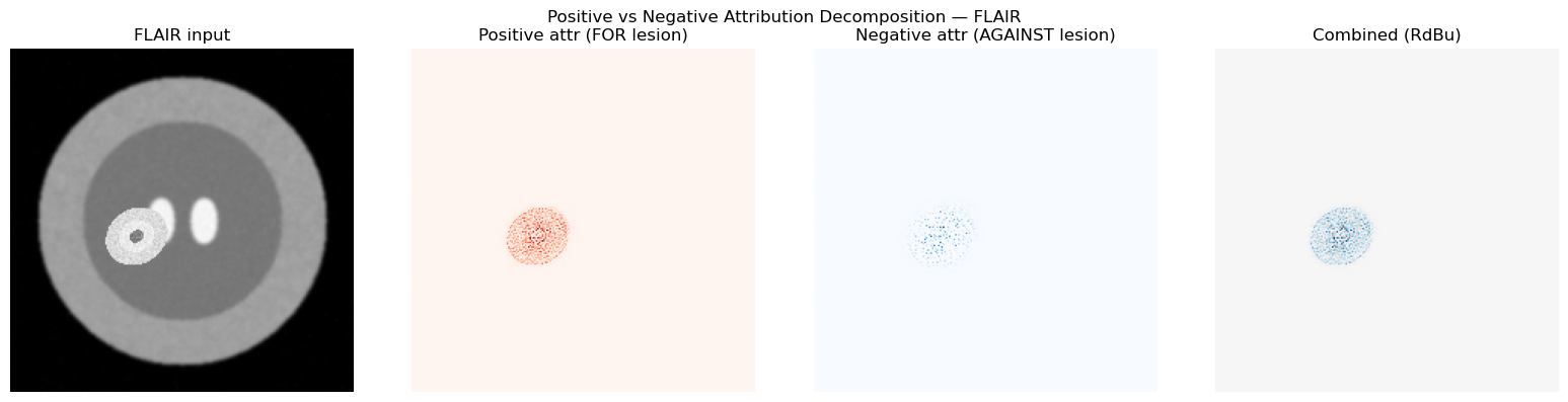
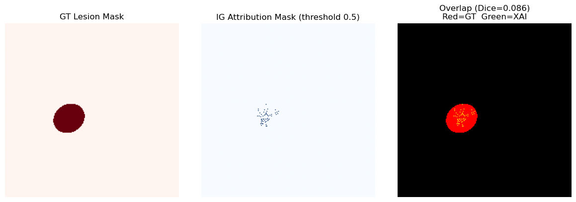
# [LIVE] Cross-Modal Consistency — Dice Overlap (XAI mask vs GT mask)

attr_norm = normalize_attr(attr_flair)
# Threshold at 50% of max
xai_mask = (attr_norm > 0.5 * attr_norm.max()).astype(np.float32)
gt_mask  = mask_xai.squeeze().numpy()

intersection = (xai_mask * gt_mask).sum()
dice_xai = 2 * intersection / (xai_mask.sum() + gt_mask.sum() + 1e-8)
print(f"Dice (IG attribution mask vs GT lesion mask): {dice_xai:.4f}")
print("Interpretation: higher Dice → attribution map clinically plausible")

fig, axes = plt.subplots(1, 3, figsize=(12, 4))
axes[0].imshow(gt_mask, cmap="Reds");  axes[0].set_title("GT Lesion Mask"); axes[0].axis("off")
axes[1].imshow(xai_mask, cmap="Blues"); axes[1].set_title("IG Attribution Mask (threshold 0.5)"); axes[1].axis("off")
overlap = np.stack([gt_mask, xai_mask, np.zeros_like(gt_mask)], axis=-1)
axes[2].imshow(overlap); axes[2].set_title(f"Overlap (Dice={dice_xai:.3f})\nRed=GT  Green=XAI"); axes[2].axis("off")
plt.tight_layout(); plt.show()
Dice (IG attribution mask vs GT lesion mask): 0.0856
Interpretation: higher Dice → attribution map clinically plausible
# Full segmentation visualization panel
fig, axes = plt.subplots(2, 4, figsize=(16, 8))

# Row 1 — inputs + masks
inputs_row = [
    (flair_xai.squeeze().detach().cpu().numpy(), "gray", "FLAIR"),
    (t1ce_xai.squeeze().detach().cpu().numpy(),  "gray", "T1ce"),
    (mask_xai.squeeze().numpy(),                  "Reds", "GT Mask"),
    (pred_mask.squeeze().detach().cpu().numpy(),  "Reds", "Predicted Mask"),
]
for ax, (im, cmap, title) in zip(axes[0], inputs_row):
    ax.imshow(im, cmap=cmap); ax.set_title(title); ax.axis("off")

# Row 2 — attribution maps
attr_row = [
    (flair_xai, attr_flair, "IG · FLAIR"),
    (t1ce_xai,  attr_t1ce,  "IG · T1ce"),
    (flair_xai, cam_flair_up, "GradCAM · FLAIR enc"),
    (t1ce_xai,  cam_t1ce_up,  "GradCAM · T1ce enc"),
]
for ax, (base_img, attr, title) in zip(axes[1], attr_row):
    ax.imshow(base_img.squeeze().detach().cpu().numpy(), cmap="gray")
    ax.imshow(normalize_attr(attr), cmap="hot", alpha=0.5)
    ax.set_title(title); ax.axis("off")

plt.suptitle("Segmentation XAI Panel — Row 1: Inputs | Row 2: Attributions", fontsize=13)
plt.tight_layout(); plt.show()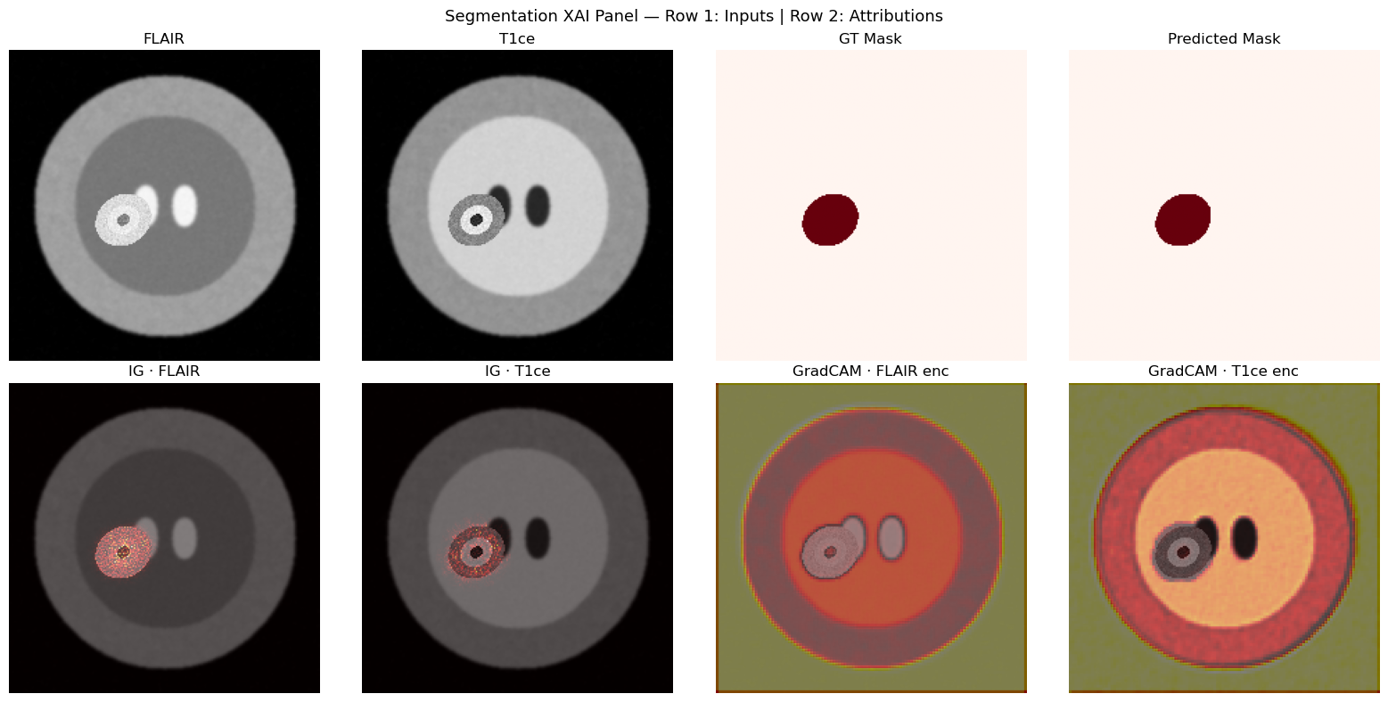
# [LIVE] Task C — XAI Gallery: IG across 6 segmentation cases
# Columns: FLAIR | FLAIR IG | T1ce | T1ce IG | GT Mask | Pred Mask

seg_model.eval()
ig_seg_gallery = IntegratedGradients(seg_xai_model)

n_gallery_seg = 6

fig, axes = plt.subplots(n_gallery_seg, 6, figsize=(22, 4 * n_gallery_seg))
col_titles = ["FLAIR", "FLAIR IG", "T1ce", "T1ce IG", "GT Mask", "Pred Mask"]
for col, ttl in enumerate(col_titles):
    axes[0, col].set_title(ttl, fontsize=10, fontweight="bold")

for row in range(n_gallery_seg):
    fl_g, t1_g, msk_g = seg_xai_ds[row]
    fl_g  = fl_g.unsqueeze(0).to(DEVICE).requires_grad_(True)
    t1_g  = t1_g.unsqueeze(0).to(DEVICE).requires_grad_(True)

    attr_fl_g, attr_t1_g = ig_seg_gallery.attribute(
        inputs=(fl_g, t1_g),
        baselines=(torch.zeros_like(fl_g), torch.zeros_like(t1_g)),
        target=0, n_steps=50,
    )
    with torch.no_grad():
        pred_msk_g = (torch.sigmoid(seg_model(fl_g, t1_g)) > 0.5).float()

    fl_np   = fl_g.squeeze().detach().cpu().numpy()
    t1_np   = t1_g.squeeze().detach().cpu().numpy()
    attr_fl = normalize_attr(attr_fl_g)
    attr_t1 = normalize_attr(attr_t1_g)
    msk_np  = msk_g.squeeze().numpy()
    pred_np = pred_msk_g.squeeze().detach().cpu().numpy()

    # Dice for this sample
    inter = (attr_fl > 0.5).astype(float) * msk_np
    dice_g = 2 * inter.sum() / ((attr_fl > 0.5).sum() + msk_np.sum() + 1e-8)

    axes[row, 0].imshow(fl_np, cmap="gray"); axes[row, 0].axis("off")
    axes[row, 0].set_ylabel(f"Case {row+1}\nDice={dice_g:.2f}", fontsize=8,
                             rotation=0, labelpad=65, va="center")

    im_fl = axes[row, 1].imshow(attr_fl, cmap="hot", vmin=0, vmax=1); axes[row, 1].axis("off")
    fig.colorbar(im_fl, ax=axes[row, 1], fraction=0.046, pad=0.04).set_label("Imp.", fontsize=6)

    axes[row, 2].imshow(t1_np, cmap="gray"); axes[row, 2].axis("off")

    im_t1 = axes[row, 3].imshow(attr_t1, cmap="hot", vmin=0, vmax=1); axes[row, 3].axis("off")
    fig.colorbar(im_t1, ax=axes[row, 3], fraction=0.046, pad=0.04).set_label("Imp.", fontsize=6)

    axes[row, 4].imshow(msk_np, cmap="Reds"); axes[row, 4].axis("off")
    axes[row, 5].imshow(pred_np, cmap="Reds"); axes[row, 5].axis("off")

fig.suptitle(
    "Task C · IG Gallery — FLAIR and T1ce attributions for 6 segmentation cases\n"
    "Dice = overlap between thresholded IG attribution mask and GT lesion mask",
    fontsize=12, y=1.01,
)
plt.tight_layout()
plt.show()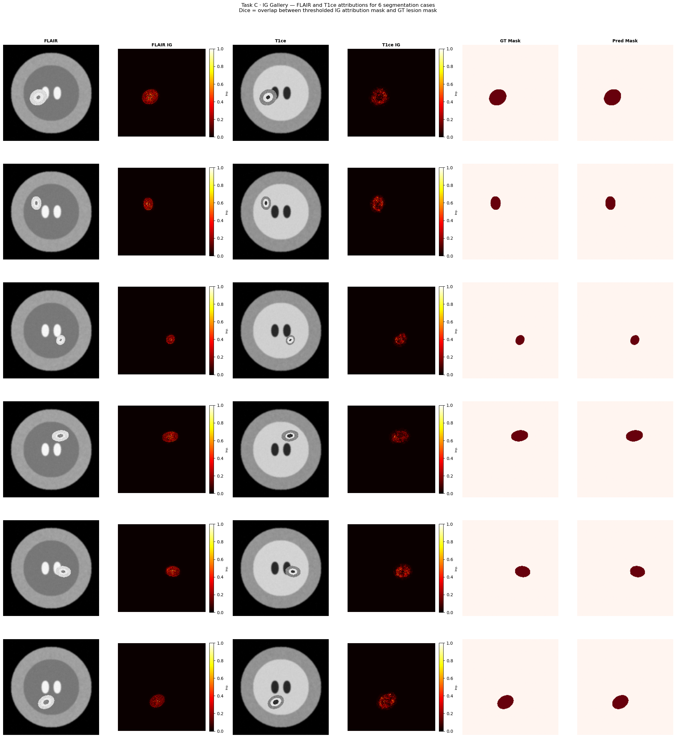
Section 7 — Clinical Validation Framework
A high-quality XAI map must satisfy four axes:
| Axis | Question | How to Assess |
|---|---|---|
| Faithfulness | Does the attribution reflect what the model actually uses? | Insertion/deletion curves, AOPC metric |
| Plausibility | Does it align with clinical domain knowledge? | Expert evaluation, annotation overlap (Dice) |
| Stability | Do small input perturbations change the attribution? | Sensitivity analysis (Pearson r > 0.95 = stable) |
| Cross-Modal | Are importance scores distributed meaningfully across modalities? | Modality importance ratio pie chart |
⚠️ XAI maps are explanations of model behavior, not ground-truth clinical markers. A model can be right for the wrong reason — always pair XAI analysis with model performance metrics.
# [LIVE] Stability / Sensitivity Test — add noise and re-compute IG
from scipy.stats import pearsonr

def stability_test(model, x1, x2, ig_method, noise_std=0.01, n_steps=50):
    """Compute Pearson r between clean and noisy IG attribution maps."""
    noisy_x1 = (x1 + noise_std * torch.randn_like(x1)).requires_grad_(True)
    noisy_x2 = (x2 + noise_std * torch.randn_like(x2)).requires_grad_(True)
    attr_clean1, _ = ig_method.attribute(
        inputs=(x1.detach().requires_grad_(True), x2.detach().requires_grad_(True)),
        baselines=(torch.zeros_like(x1), torch.zeros_like(x2)),
        target=0, n_steps=n_steps,
    )
    attr_noisy1, _ = ig_method.attribute(
        inputs=(noisy_x1, noisy_x2),
        baselines=(torch.zeros_like(noisy_x1), torch.zeros_like(noisy_x2)),
        target=0, n_steps=n_steps,
    )
    r, _ = pearsonr(
        attr_clean1.flatten().detach().numpy(),
        attr_noisy1.flatten().detach().numpy(),
    )
    return r


# Segmentation stability (FLAIR modality)
r_seg = stability_test(seg_xai_model, flair_xai.cpu(), t1ce_xai.cpu(), ig_seg, noise_std=0.01)
print(f"Segmentation IG stability (Pearson r): {r_seg:.4f}  [ideal: > 0.95]")

# Regression stability (T1 modality)
r_reg = stability_test(reg_model, t1_xai.cpu(), t2_xai.cpu(), ig_reg, noise_std=0.01)
print(f"Regression   IG stability (Pearson r): {r_reg:.4f}  [ideal: > 0.95]")
Segmentation IG stability (Pearson r): 0.9231 [ideal: > 0.95]
Regression IG stability (Pearson r): 0.1706 [ideal: > 0.95]
import pandas as pd

summary_data = [
    # Task A — Classification
    {"Task": "Classification", "Method": "Integrated Gradients", "Runtime": "Medium", "Stability": "High", "Spatial Res.": "Full", "Multi-Input": "✓"},
    {"Task": "Classification", "Method": "DeepLIFT",             "Runtime": "Fast",   "Stability": "High", "Spatial Res.": "Full", "Multi-Input": "✓"},
    {"Task": "Classification", "Method": "GradientSHAP",         "Runtime": "Slow",   "Stability": "Medium","Spatial Res.": "Full", "Multi-Input": "✓"},
    {"Task": "Classification", "Method": "LayerGradCAM",         "Runtime": "Fast",   "Stability": "Medium","Spatial Res.": "Low (layer)", "Multi-Input": "Image only"},
    {"Task": "Classification", "Method": "Occlusion",            "Runtime": "Very slow","Stability":"High","Spatial Res.": "Patch-level","Multi-Input": "✓"},
    # Task B — Regression
    {"Task": "Regression",     "Method": "Integrated Gradients", "Runtime": "Medium", "Stability": "High", "Spatial Res.": "Full", "Multi-Input": "✓"},
    {"Task": "Regression",     "Method": "DeepLIFT",             "Runtime": "Fast",   "Stability": "High", "Spatial Res.": "Full", "Multi-Input": "✓"},
    {"Task": "Regression",     "Method": "Saliency",             "Runtime": "Fast",   "Stability": "Low",  "Spatial Res.": "Full", "Multi-Input": "✓"},
    {"Task": "Regression",     "Method": "Feature Ablation",     "Runtime": "Slow",   "Stability": "High", "Spatial Res.": "Modality-level","Multi-Input": "✓"},
    # Task C — Segmentation
    {"Task": "Segmentation",   "Method": "IG + SegWrapper",      "Runtime": "Medium", "Stability": "High", "Spatial Res.": "Full", "Multi-Input": "✓"},
    {"Task": "Segmentation",   "Method": "LayerGradCAM (dual)",  "Runtime": "Fast",   "Stability": "Medium","Spatial Res.": "Low (layer)","Multi-Input": "✓ (per branch)"},
]

df = pd.DataFrame(summary_data)
display(df.style.set_caption("XAI Method Comparison Across All Three Tasks"))
print(df.to_string(index=False)) Task Method Runtime Stability Spatial Res. Multi-Input
Classification Integrated Gradients Medium High Full ✓
Classification DeepLIFT Fast High Full ✓
Classification GradientSHAP Slow Medium Full ✓
Classification LayerGradCAM Fast Medium Low (layer) Image only
Classification Occlusion Very slow High Patch-level ✓
Regression Integrated Gradients Medium High Full ✓
Regression DeepLIFT Fast High Full ✓
Regression Saliency Fast Low Full ✓
Regression Feature Ablation Slow High Modality-level ✓
Segmentation IG + SegWrapper Medium High Full ✓
Segmentation LayerGradCAM (dual) Fast Medium Low (layer) ✓ (per branch)
Key Takeaways
1 · XAI Taxonomy Mastery
You covered all three families: gradient-based (IG, DeepLIFT, GradSHAP, GradCAM), perturbation-based (Occlusion, Feature Ablation), and know where attention-based fits.
2 · Multi-Modal Fusion Analysis
The modality importance ratio (pie chart from IG abs-mean) is a powerful clinical communication tool: it quantifies which imaging channel drove the decision in plain language.
3 · Captum Proficiency — Three Key Patterns
Tuple-input API:
ig.attribute(inputs=(x1, x2), baselines=(b1, b2))Wrapper pattern:
MultiInputWrapperandSegReductionWrapperfor Captum compatibilitySegmentation reduction: collapse
(B,1,H,W)→(B,1)before attribution
4 · Clinical Validation — Four Axes
| Axis | Quick Test |
|---|---|
| Faithfulness | Does removing high-attribution regions drop confidence? |
| Plausibility | Does the heatmap match the planted signal region? (Dice overlap) |
| Stability | Pearson r > 0.95 between clean and noisy attribution maps |
| Cross-Modal | Modality importance ratio consistent with known data structure |
⚠️ Warning: XAI maps explain model behavior, not clinical ground truth. A perfectly faithful explanation of a poorly trained model is still clinically useless.
Next Steps & Extensions
Real data (v0.6): Replace dummy generators with SIIM-ISIC (classification), OSIC (regression), LGG MRI (segmentation) — all available on Kaggle with drop-in compatible loaders
Stronger encoders: ResNet-18 / EfficientNet-B0 frozen backbone + fine-tuned fusion head
Attention-based XAI: Transformer cross-attention maps, DINO self-supervised features
Captum Insights: Interactive dashboard for exploratory attribution analysis
AOPC / insertion-deletion curves: Quantitative faithfulness benchmarks